chapter. Unstructured Finite Volume Schemes 第5章 非结构网格有限体积格式[cfd-0006]
正如我们在第3章引言中已经指出的ï¼求解欧拉方程和Navier-Stokes方程的绝大多数数值格式都采用线方法(method of lines)ï¼即在空间和时间上分别离散化。这种方法的主要优点是:允许我们对空间导数和时间导数选用不同精度的数值近似。与基于空间-时间耦合(coupled)离散化的方法——如Lax-Wendroff格式族(例如显式MacCormack预估-校正格式、隐式Lerat格式等ï¼细节可参见文献[1])——相比ï¼这带来了大得多的灵活性。由于线方法的广泛应用ï¼本书在此也遵循这一路线。en
As we already noted in the introduction to Chapter 3, the vast majority of numerical schemes for the solution of the Euler- and the Navier-Stokes equations employs the method of lines, i.e., a separate discretisation in space and in time. The main advantage of this approach is that it allows us to select numerical approximations of different accuracy for the spatial and temporal derivatives. This offers a significantly larger flexibility as compared to methods based on coupled space and time discretisation, like the Lax-Wendroff family of schemes (e.g., explicit MacCormack predictor-corrector scheme, implicit Lerat's scheme, etc. - details may be found, e.g., in Ref. [1]). Because of the popularity of the method of lines, we shall follow this approach here.
本章讨论的有限体积格式建立在守恒定律的基础上ï¼即由Navier-Stokes方程(2.19)或欧拉方程(2.45)所表示的守恒定律。在前处理步骤中ï¼首先把物理域划分成若干元素(网格单元)。在二维情形ï¼元素为三角形ï¼有时与四边形组合使用。在三维情形ï¼最常采用的是四面体[2]-[7]。然而ï¼越来越多的流动求解器在模拟高雷诺数黏性流动时ï¼采用四面体、棱柱、四棱锥的混合ï¼某些情形还包括六面体(图5.1)[8]-[16]。由多种单元类型构成的非结构网格称为混合网格(mixed grids)。例子见图3.3和图5.2。“混合网格”这一名称不应与术语杂交网格(hybrid grids)相混淆ï¼后者指结构-非结构组合网格(例如[17]-[19])。en
The finite volume schemes, which are discussed in this chapter, are based on the conservation laws, as they are represented by the Navier-Stokes (2.19) or by the Euler equations (2.45). In a pre-processing step, the physical domain is first subdivided into a number of elements (grid cells). In two dimensions, the elements are triangles, sometimes combined with quadrilaterals. In three dimensions, tetrahedra are most often employed [2]-[7]. However, an increasing number of flow solvers uses a mix of tetrahedra, prisms, pyramids, and in some cases also hexahedra (Fig. 5.1) for the simulation of high Reynolds number viscous flows [8]-[16]. Unstructured grids composed of various cell types are referred to as mixed grids. Examples are provided in Figs. 3.3 and 5.2. The designation 'mixed grids' should not be confused with the term hybrid grids, which means combined structured-unstructured grids (e.g., [17]-[19]).
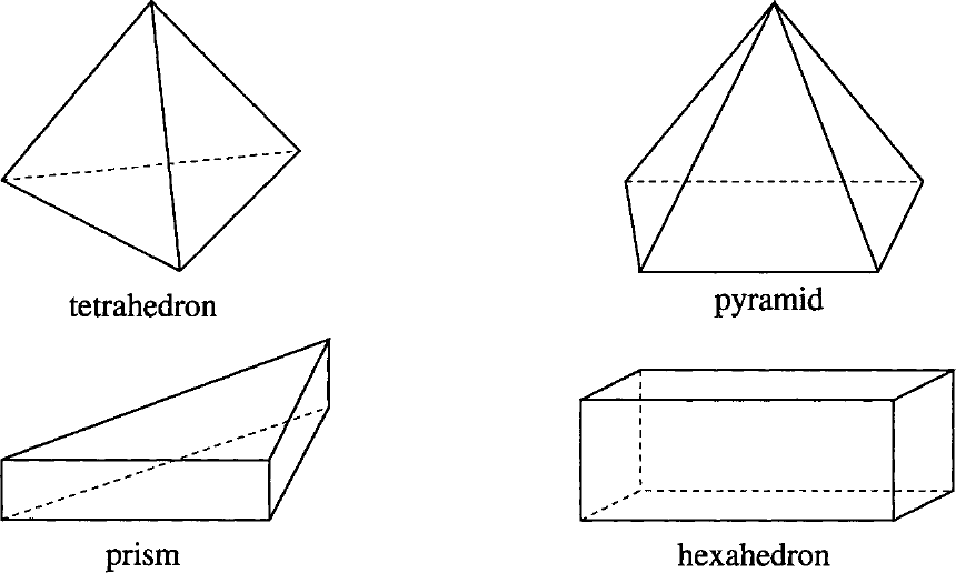
图5.1:用于生成三维非结构网格的单元(elements)。图例:四种单元分别为四面体(tetrahedron)、四棱锥(pyramid)、棱柱(prism)和六面体(hexahedron)。
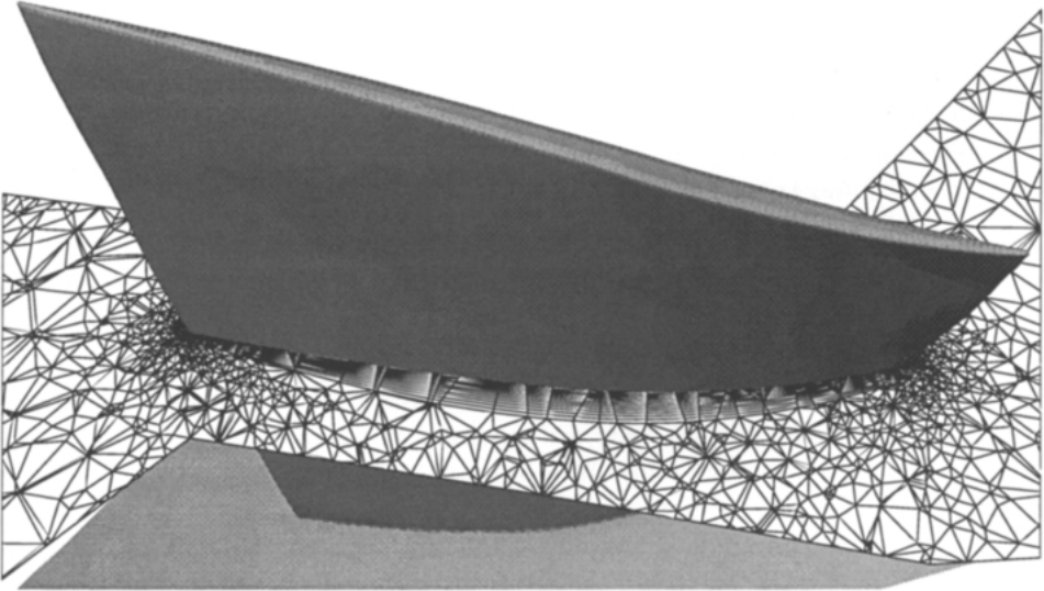
图5.2:绕压气机叶片的三维非结构混合网格的平面剖切。网格由CENTAUR™[20]、[21]生成。图例:注意绕叶身表面的四边形面层ï¼它由棱柱单元形成;四面体网格的不规则性由平面剖切造成。
网格生成必须以保持控制方程守恒性质的方式进行ï¼即:
- 物理域必须被网格完全覆盖;
- 元素之间不得留有空隙;
- 各元素不得相互重叠。
en
The grid generation has to be done in a way that preserves the conservation properties of the governing equations, namely:
- the physical domain has to be completely covered by the grid,
- there must be no free space left between the elements,
- the elements may not overlap.
除满足上述要求之外ï¼网格还应当是光滑的ï¼即相邻网格单元的体积或拉伸比不应相差悬殊ï¼且元素应尽可能规则。否则ï¼数值误差可能完全破坏解的精度[22]、[23]。en
In addition to fulfilling the above requirements, the grid should be smooth, i.e., there should be no large differences in the volumes or in the stretching ratio of adjacent grid cells and the elements should be as regular as possible. Otherwise, the numerical errors could spoil the solution accuracy completely [22], [23].
在网格的基础上定义适当的控制体ï¼以便计算对流通量、黏性通量以及源项的积分。为简单起见ï¼假设某一控制体不随时间变化(否则参见附录A.5)。于是ï¼守恒变量\(\vec{W}\)的时间导数可以写成en
Based on the grid, suitable control volumes are defined in order to evaluate the integrals of the convective and viscous fluxes as well as of the source term. For simplicity, let us assume that a particular control volume does not change in time (otherwise see Appendix A.5). Then, the time derivative of the conservative variables \(\vec{W}\) can be cast in the form
由此ï¼方程(2.19)变为en
Herewith, Eq. (2.19) becomes
方程(5.1)右端的面积分ï¼用穿过控制体各面的通量之和来近似。这一近似称为空间离散化(spatial discretisation)。通常假设通量沿每个面为常数ï¼并在面的中点处取值。这一处理对二阶精度格式已经足够。源项一般假设在控制体内部为常数。然而ï¼当源项占主导地位时ï¼建议把\(\vec{Q}\)取为相邻控制体上数值的加权和(参见[24]及其所引文献)。如果考虑某个具体的控制体\(\Omega_I\)ï¼则由方程(5.1)得到en
The surface integral on the right-hand side of Equation (5.1) is approximated by a sum of the fluxes crossing the faces of the control volume. This approximation is called spatial discretisation. It is usually supposed that the flux is constant along the individual face and that it is evaluated at the midpoint of the face. This treatment is sufficient for a second-order accurate scheme. The source term is generally assumed to be constant inside the control volume. However, in cases where the source term becomes dominant, it is advisable to evaluate \(\vec{Q}\) as the weighted sum of values from the neighbouring control volumes (see [24] and the references cited therein). If we consider a particular volume \(\Omega_I\), we obtain from Eq. (5.1)
在上式中ï¼大写指标\(I\)指代控制体ï¼因为一般来说控制体并不一定与网格重合ï¼这一点稍后会看到。此外,\(N_F\)表示控制体\(\Omega_I\)的面数ï¼变量\(\Delta S_m\)代表第\(m\)个面的面积。面数\(N_F\)当然取决于单元类型ï¼但也取决于控制体的类型。一般而言ï¼不同控制体的面数也各不相同ï¼这是与结构网格相比的主要区别之一。不过ï¼人们已发展出无需预先知道\(N_F\)的数值方法和数据结构ï¼我们将在后面的章节再回到这一点。en
In the above expression, the index \(I\) in capital letters references the control volume, since in general it does not necessarily coincide with the grid, as we shall see later. Furthermore, \(N_F\) denotes the number of the faces of the control volume \(\Omega_I\), and the variable \(\Delta S_m\) stands for the area of the face \(m\), respectively. The number of faces \(N_F\) depends of course on the cell-type but also on the type of the control volume. In general, the number of faces changes between the control volumes as well, which is one of the main differences as compared to structured grids. However, numerical procedures and data structures were developed which avoid the a priori knowledge of \(N_F\). We shall return to this point in later sections.
对所有控制体\(\Omega_I\)写出方程(5.3)的关系式ï¼便得到一阶常微分方程组。这些方程在时间上是双曲型的ï¼这意味着必须从已知的初始解出发沿时间推进求解。我们还必须为黏性通量和无黏通量提供适当的边界条件ï¼如第8章所述。en
Writing down the relationship in Equation (5.3) for all control volumes \(\Omega_I\), we obtain a system of ordinary differential equations of first order. The equations are hyperbolic in time, that means we have to advance them in time starting from a known initial solution. We have also to provide appropriate boundary conditions for the viscous and the inviscid fluxes, as they are described in Chapter 8.
在数值求解离散化控制方程组(5.3)时ï¼第一个问题是如何定义控制体ï¼以及相对于网格点把流动变量布置在何处。在有限体积格式的框架下ï¼可以采取三种基本策略:
- 单元中心格式(cell-centred scheme)[25]、[26]、[2]、[16]——控制体与网格单元完全相同ï¼流动变量布置在各单元的形心处(图5.6)。
- 采用重叠(overlapping)控制体的单元顶点格式(cell-vertex scheme)[27]、[28]——流动量被赋给网格顶点ï¼控制体定义为共享相应节点的所有网格单元的并集。这意味着与两个相邻顶点相对应的控制体彼此重叠。
- 采用中位对偶(median-dual)控制体的单元顶点格式[29]-[33]、[13]、[15]——流动变量同样存储在网格顶点上ï¼但此时控制体由连接周围各元素的形心、面形心和边中点而构成(图5.7、图5.8)。这样ï¼每个网格点都被其对应的控制体所包围——构成一幅对偶网格(dual grid)——且各控制体互不重叠。
en
When numerically solving the system of discretised governing equations (5.3), the first question is how to define the control volumes and where to locate the flow variables with respect to the grid points. In the framework of finite volume schemes, three basic strategies can be pursued:
- Cell-centred scheme [25], [26], [2], [16] - control volumes are identical with the grid cells and the flow variables are associated with their centroids (Fig. 5.6).
- Cell-vertex scheme with overlapping control volumes [27], [28] - flow quantities are assigned to the grid vertex and the control volumes are defined as the union of all grid cells having the respective node in common. This means that the control volumes associated with two neighbouring vertices overlap each other.
- Cell-vertex scheme with median-dual control volumes [29]-[33], [13], [15] - flow variables are again stored at the grid vertices, but the control volumes are now created by connecting the centroids of the surrounding elements, face-centroids and edge-midpoints (Figs. 5.7, 5.8). In this way, the grid points are encapsulated by their corresponding control volumes - representing a dual grid - which do not overlap.
由于采用重叠控制体的单元顶点格式已不再使用ï¼这里集中讨论单元中心格式和中位对偶格式。两种方法都将在5.2节中详细讨论。en
Because the cell-vertex scheme with overlapping control volumes is no longer used, we shall concentrate here on the cell-centred and on the median-dual scheme. Both methodologies will be discussed in detail in Section 5.2.
需要注意的是ï¼在我们的情形中ï¼所有流动变量——即守恒变量\((\rho, \rho u, \rho v, \rho w\)与\(\rho E)\)以及因变量\((p, T, c\)等)——都布置在同一位置:或在单元中心ï¼或在网格点。这一做法称为同位网格(co-located grid)方案。与此相反ï¼许多较老的(结构网格)基于压力的方法(参见3.1节)采用所谓的交错网格(staggered grid)方案ï¼把压力和速度分量存储在不同位置ï¼以抑制中心差分所引起的解的振荡。en
It is important to notice that in our case all flow variables, i.e., the conservative variables \((\rho, \rho u, \rho v, \rho w\) and \(\rho E)\) and the dependent variables \((p, T, c\), etc.), are associated with the same location - with the cell centre or with the grid point. This approach is known as the co-located grid scheme. By contrast, many older (structured) pressure-based methods (cf. Section 3.1) use the so-called staggered grid scheme, where the pressure and the velocity components are stored at different locations in order to suppress oscillations of the solution which arise from central differencing.
在对流通量的计算方面存在许多选择。基本问题在于:我们必须知道控制体全部\(N_F\)个面上的通量值ï¼但流动变量在这些面上并不能直接得到。这意味着ï¼我们必须把通量或流动变量插值到控制体的面上。流动变量的插值称为由控制体内部之值对解的重构(reconstruction)(参见5.3.3小节)。原则上ï¼插值可以按以下两种方式之一进行:
- 像中心(central)离散格式那样ï¼采用算术平均;
- 像上风(upwind)离散格式那样ï¼采用某种偏置插值ï¼以照顾流动方程的特征(方向)。
en
Many choices exist with respect to the evaluation of the convective fluxes. The basic problem is that we have to know their values at all \(N_F\) faces of a control volume, but the flow variables are not directly available there. This means, we have to interpolate either the fluxes or the flow variables to the faces of the control volume. The interpolation of flow variables is known as reconstruction of the solution from values inside the control volumes (see Subsection 5.3.3). In principle, the interpolation can be conducted in one of two ways:
- by arithmetic averaging like in central discretisation schemes;
- by some biased interpolation like in upwind discretisation schemes, which take care of the characteristics of the flow equations.
除描述这些格式之外ï¼我们还将在5.3节讨论最常用的对流通量离散格式的精度、适用范围和计算量等方面。en
Besides the description, we shall treat aspects such as accuracy, range of applicability and numerical effort of the most widely used discretisation schemes for the convective fluxes in Section 5.3.
在控制体某个面上计算黏性通量的一种常用方法ï¼基于流动量的算术平均。更为复杂的是方程(2.15)和(2.24)中速度梯度与温度梯度的计算ï¼在混合网格的情形下尤其如此。我们将在5.4节给出完整的处理流程。en
A commonly applied methodology for the evaluation of the viscous fluxes at a face of the control volume is based on arithmetic averaging of the flow quantities. More involved is the calculation of the velocity and the temperature gradients in Equations (2.15) and (2.24), particularly in the case of mixed grids. We shall present the complete procedure in Section 5.4.
5.1 Geometrical Quantities of a Control Volume 控制体的几何量[cfd-5-1]
在开始讨论作用于对流通量和黏性通量的离散化方法之前ï¼重要的是先考虑控制体\(\Omega_I\)各几何量的计算——即它的体积、单位法向量\(\vec{n}_m\)(定义为指向外侧)、面\(m\)的面积\(\Delta S_m\)ï¼以及元素的形心。法向量与面面积也合称为控制体的度量(metrics)。下面我们分别讨论二维和三维情形。en
Before we start to discuss the discretisation methodologies applied to the convective and viscous fluxes, it is important to consider the evaluation of geometrical quantities of the control volume \(\Omega_I\) - its volume, the unit normal vector \(\vec{n}_m\) (defined as outward facing) and the area \(\Delta S_m\) of a face \(m\), as well as the centroid of an element. The normal vector and the face area are also denoted as the metrics of the control volume. In the following, we shall consider the 2-D and the 3-D case separately.
5.1.1 Two-Dimensional Case 二维情形[cfd-5-1-1]
一般而言ï¼我们把平面内的流动看作三维问题的一种特殊情形ï¼其中解关于某一坐标方向(例如\(z\)方向)对称。由于对称性ï¼也为了得到体积、压力等量的正确物理单位ï¼我们把所有网格单元和控制体的深度设为常数\(b\)。于是ï¼在二维情形ï¼控制体的体积等于其面积与深度\(b\)的乘积。由于深度\(b\)是任意的ï¼为方便起见可取\(b = 1\)。在下面的讨论中ï¼我们只考虑三角形和四边形元素。尽管中位对偶格式的控制体形状可能相当复杂ï¼但它总可以分解为三角形和/或四边形。en
Generally, we think of the flow in a plane as being a special case of a 3-D problem, where the solution is symmetric with respect to one coordinate direction (e.g., to the \(z\)-direction). Because of the symmetry and in order to obtain correct physical units for volume, pressure, etc., we set the depth of all grid cells and control volumes equal to a constant value \(b\). The volume of a control volume results then in 2D from the product of its area with the depth \(b\). Since the depth \(b\) is arbitrary, we may set \(b = 1\) for convenience. In the following discussion, we restrict ourselves to triangular and quadrilateral elements. Even though the control volume of a median-dual scheme can have a rather complex shape, it can always be decomposed into triangles and/or quadrilaterals.
Triangular element 三角形元素
一般三角形的面积可以用高斯(Gauss)公式最方便且精确地计算。于是ï¼采用图5.3a所示的节点编号ï¼体积由下式给出en
The area of a general triangle can be most conveniently and exactly calculated by the formula of Gauss. Thus, using a node numbering in accordance with Fig. 5.3a, the volume results from
节点必须按逆时针方向编号ï¼才能得到正的体积值。en
The nodes have to be numbered in the anti-clockwise direction in order to obtain a positive value for the volume.
Quadrilateral element 四边形元素
一般四边形的面积可以用高斯公式精确计算ï¼经过一些代数运算后得到表达式en
The area of a general quadrilateral can be exactly calculated by Gauss' formula, which leads, after some algebra, to the expression
其中节点按图5.3b沿逆时针方向编号。上式中ï¼我们假定控制体位于\(x-y\)平面内,\(z\)坐标为对称轴。en
where the nodes are numbered according to Fig. 5.3b in the anti-clockwise direction. In the above, we assumed that the control volume is located in the \(x-y\)-plane and that the \(z\)-coordinate represents the symmetry axis.
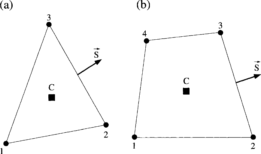
图5.3:节点编号与面向量:(a)三角形元素;(b)四边形元素。C表示元素的(几何)中心。
在二维情形ï¼控制体的各条边均为直线ï¼因此单位法向量沿边保持不变。当我们按照方程(5.2)的近似对通量进行积分时ï¼需要计算面的面积\(\Delta S\)与相应单位法向量\(\vec{n}\)的乘积ï¼即面向量(face vector)\(\vec{S}\)。参照图5.3ï¼例如边2-3处的外指面向量由下式给出en
The edges of a control volume are given by straight lines in 2D and therefore the unit normal vector is constant along them. When we integrate the fluxes according to the approximation of Eq. (5.2), we have to evaluate the product of the area of a face \(\Delta S\) and the corresponding unit normal vector \(\vec{n}\) which is the face vector \(\vec{S}\). Considering Fig. 5.3, the outward pointing face vector, e.g., at the side 2-3 is given by
其中\(S_x\)、\(S_y\)为面向量的笛卡尔分量。en
where \(S_x\), \(S_y\) denote the Cartesian components of the face vector.
Element Centre 单元中心
图5.3a中三角形的中心定义为en
The centre of the triangle from Fig. 5.3a is defined as
其中\(\vec{r}_{1/2/3}\)表示各节点的笛卡尔坐标。四边形元素的中心可用文献[34]中给出的公式计算。为此ï¼把四边形分解为共享两个点的两个三角形。按图5.3b的节点编号ï¼并取1和3为公共节点ï¼该关系式为en
with \(\vec{r}_{1/2/3}\) representing the Cartesian coordinates of the nodes. The centre of a quadrilateral element can be computed by the formula given in Ref. [34]. For this purpose, the quadrilateral is decomposed into two triangles which share two points. With the node numbering according to Fig. 5.3b, and 1 and 3 being the common nodes, the relation reads
5.1.2 Three-Dimensional Case 三维情形[cfd-5-1-2]
与前面的二维情形不同ï¼在三维情形ï¼对具有四边形面的元素或控制体计算面向量和体积会遇到一些问题。主要原因在于ï¼控制体四边形面的四个顶点一般不一定位于同一平面内。此时ï¼法向量在这样的面上不再是常数(见图4.2)。为克服这一困难ï¼可以把每个四边形面分解成两个甚至更多的三角形。然而ï¼对光滑网格上的二阶格式而言ï¼精度上的收益几乎察觉不到。这种额外的代价只有对三阶及更高阶空间离散化才是值得的——实际上也是必需的。因此ï¼在下面的讨论中ï¼我们将对四边形面采用一种基于平均法向量的简化处理方法。en
As opposed to the previous 2-D case, the computation of face vectors and volumes poses in 3D some problems for elements or control volumes with quadrilateral faces. The main reason for this is that, in general, the four vertices of a quadrilateral face of a control volume may not lie in a plane. Then, the normal vector is no longer constant on such face (see Fig. 4.2). In order to overcome this difficulty, we could decompose each quadrilateral face into two or even more triangles. However, the gain in accuracy is hardly noticeable for a second-order scheme on a smooth grid. The additional effort can only be justified - and in fact it becomes necessary - for a third- and higher order spatial discretisations. Therefore, we shall apply a simplified treatment of the quadrilateral faces in the following considerations, which is based on an averaged normal vector.
Triangular face 三角形面
对于三角形面ï¼面向量\(\vec{S}\)可以用高斯公式精确计算。按图5.4a定义节点ï¼对三角形1-2-3的边差分得到en
The face vector \(\vec{S}\) can be exactly computed for a triangular face using Gauss' formula. Defining the nodes according to Fig. 5.4a, we obtain for the edge differences of the triangle 1-2-3
于是ï¼外指面向量\(\vec{S} = \vec{n}\Delta S\)由下式得到en
The outward pointing face vector \(\vec{S} = \vec{n}\Delta S\) results then from
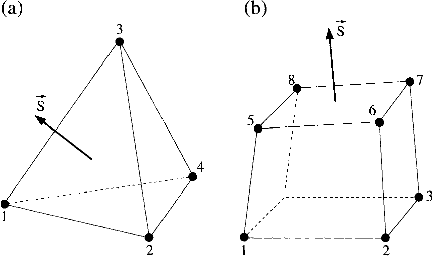
图5.4:节点编号与面向量:(a)四面体元素;(b)六面体元素。图例:(a)中节点1—4为四面体的顶点,\(\vec{S}\)为面向量;(b)中节点1—8为六面体的顶点,\(\vec{S}\)为面5-6-7-8上的外指面向量。
Quadrilateral face 四边形面
四边形面(诸如图5.4b所示的面)的平均面向量\(\vec{S}\)ï¼最方便是采用与二维情形计算四边形面积相同的高斯公式来计算。于是ï¼对于图5.4b中由节点5、6、7和8给出的面ï¼首先定义如下差分en
The averaged face vector \(\vec{S}\) of a quadrilateral face, like that rendered in Fig. 5.4b, is most conveniently computed using the same Gauss' formula as employed in 2-D for the area of a quadrilateral. Thus, for the face given by the nodes 5, 6, 7 and 8 in Fig. 5.4b, we first define the differences
然后ï¼由下述关系式得到外指面向量\(\vec{S} = \vec{n}\Delta S\)en
Then, we obtain the outward pointing face vector \(\vec{S} = \vec{n}\Delta S\) from the relation
当面接近平行四边形ï¼即面的四个顶点全部位于同一平面内时ï¼这一近似变为精确的。en
The approximation becomes exact when the face approaches a parallelogram, i.e., when the vertices of the face lie all in one plane.
两种情形下的单位法向量都由\(\vec{n} = \vec{S}/\Delta S\)得到ï¼其中en
The unit normal vector is obtained in both cases from \(\vec{n} = \vec{S}/\Delta S\) with
Volume 体积
正如在三维结构网格有限体积格式的情形中已经指出的ï¼体积的一种非常方便的计算方法基于散度定理(divergence theorem)[35]。4.1.2小节的讨论最终给出表达式en
As we already stated in the case of 3-D structured finite volume schemes, a very convenient approach for the computation of volumes is based on the divergence theorem [35]. The discussion in Subsection 4.1.2 led finally to the expression
此即体积的表达式ï¼其中\(N_F\)表示控制体的面数,\((\vec{r}_c)_m\)为控制体第\(m\)个面的中心,\(\vec{S}_m\)为第\(m\)个面(外指)的面向量。公式(5.15)可直接应用于非结构网格。对于所有面均为三角形、或四边形面均为平面的体积ï¼该公式是精确的。en
for the volume, where \(N_F\) denotes the number of the faces of the control volume, \((\vec{r}_c)_m\) the centre of the face \(m\) of the control volume, and \(\vec{S}_m\) the face vector (outward directed) of the face \(m\), respectively. The formula (5.15) is directly applicable on unstructured grids. It is exact for a volume with triangular faces, or a volume with planar quadrilateral faces.
Cell Centroid 单元形心
前面提到的中位对偶型控制体需要知道网格单元的形心。一般体积的形心定义为en
The previously mentioned median-dual type of control volume requires the knowledge of the centroid of the grid cell. The centroid of a general volume is defined as
5.2 General Discretisation Methodologies 一般离散化方法[cfd-5-2]
我们在本章开头已经提到ï¼在控制体的定义和流动变量的布置方面有两种常用的做法:单元中心格式和中位对偶格式。本节将对两者作更详细的介绍。en
We already mentioned at the beginning of this chapter that there are two popular approaches for the definition of the control volume and for the location of the flow variables. These are the cell-centred scheme and the median-dual scheme. We shall present both in more detail in this section.
不过ï¼在开始之前ï¼先简要谈一谈非结构流动求解器所需的基本数据结构。事实上ï¼一个灵活而在内存和运算量方面又高效的数据结构ï¼是任何非结构格式的关键所在。可以说ï¼网格中所缺失的结构必须在求解器内部来提供。至少需要以下数据:
- 网格节点(顶点)的坐标;
- 从元素指向网格节点的指针;
- 从位于边界上的元素面指向网格节点的指针。
en
However, before we start, let us say a few words about the basic data structure which is needed for an unstructured flow solver. In fact, a flexible but in terms of memory and operation count efficient data structure is the crucial point of any unstructured scheme. You can say that the structure which is missing in the grid has to be provided inside the solver. At least the following data is required:
- coordinates of the grid nodes (vertices),
- pointers from elements to grid nodes,
- pointers from faces of elements located on a boundary to grid nodes.
离散格式所需的进一步数据结构可以由这些信息生成。为说明上述数据可能如何存储ï¼让我们以图5.4a中的四面体为例。如果进一步假设面1-2-4位于某一边界(壁面、入口、远场等)上ï¼则可以采用如下格式:en
Further data structures, which are required by the discretisation schemes, can be generated from this information. In order to illustrate how the above data could possibly be stored, let us consider for example the tetrahedron in Fig. 5.4a. If we further assume that the face 1-2-4 is on a boundary (wall, inlet, farfield, etc.), we could employ the format:
# nodes (x, y, z):
  P1.x  P1.y  P1.z
  P2.x  P2.y  P2.z
  P3.x  P3.y  P3.z
  P4.x  P4.y  P4.z
  ...
# tetrahedra:
  ...
  P1  P2  P3  P4
  ...
# boundaries:
  ...
  type  P1  P4  P2
  ...
随书CD-ROM所附的二维非结构代码也采用类似的格式。en
A similar format is also utilised by the 2-D unstructured code provided on the accompanying CD-ROM.
关于计算域的边界ï¼认识到以下两点十分重要。第一ï¼存储边界面比只存储(边界)节点更为方便。考察图5.5所示的情景即可理解这一点。问题在于:节点\(P_1\)被三条边界共享ï¼节点\(P_2\)和\(P_3\)被两条物理类型可能不同的边界共享。因此ï¼施加正确的边界条件可能变得非常繁琐。相反ï¼一个面只能属于一条边界ï¼例如\(P_1-P_2-P_4\)属于边界1。en
It is important to realise the following two points related to the boundaries of the computational domain. First, it is more convenient to store boundary faces than just the nodes. This can be understood by considering the situation depicted in Fig. 5.5. The problem is that node \(P_1\) is shared by three, nodes \(P_2\) and \(P_3\) by two boundaries of possibly physically different types. Therefore, it can become very cumbersome to apply the correct boundary conditions. On the contrary, a face can belong to only one boundary, like \(P_1-P_2-P_4\) to boundary 1.
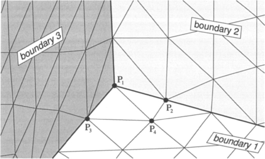
图5.5:相交于一个角点的三条边界——网格点相对于边界类型的二义性(ambiguity)。图例:三条边界分别标记为boundary 3、boundary 2、boundary 1;节点\(P_1\)、\(P_2\)、\(P_3\)位于边界交汇处附近,\(P_4\)为相邻内部节点;面\(P_1-P_2-P_4\)属于边界1。
5.2.1 Cell-Centred Scheme 单元中心格式[cfd-5-2-1]
如果控制体与网格单元完全相同ï¼且流动变量布置在各单元的形心处(如图5.6所示)ï¼我们就称之为单元中心格式。在计算离散化流动方程(5.2)时ï¼需要在控制体各面的中点处提供对流通量和黏性通量ï¼这对光滑网格上的二阶精度离散化已经足够(四边形面采用平均法向量)。通量可以用以下三种方式之一来近似:
- 通量平均(average of fluxes):由单元面左右两侧网格单元形心处之值分别计算通量ï¼再取平均ï¼但使用同一单位法向量(一般只用于对流通量);
- 变量平均(average of variables):采用单元面左右两侧相邻网格单元形心处变量的平均;
- 由周围单元之值分别在单元面两侧重构(reconstructed)流动量ï¼再由此计算通量(只用于对流通量)。
en
We speak of a cell-centred scheme if the control volumes are identical with the grid cells and if the flow variables are associated with their centroids, as it is sketched in Fig. 5.6. When we evaluate the discretised flow equations (5.2), we have to supply the convective and the viscous fluxes at the midpoints of the faces of the control volume, which is sufficient for a second-order accurate discretisation on smooth grids (averaged normal vector is employed for quadrilateral faces). The fluxes can be approximated in one of three ways:
- by the average of fluxes computed from values at the centroids of the grid cells to the left and to the right of the cell face, but using the same unit normal vector (generally applied only to the convective fluxes);
- by using an average of variables associated with the centroids of the grid cells adjacent to the left and to the right side of the cell face;
- by computing the fluxes from flow quantities reconstructed separately on both sides of the cell face from values in the surrounding cells (employed only for the convective fluxes).
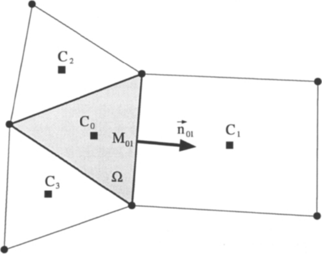
图5.6:单元中心格式的控制体(二维)。图例:网格节点用圆点表示ï¼单元中心用方块(C)表示;\(C_0\)、\(C_1\)、\(C_2\)、\(C_3\)为相邻单元的形心,\(M_{01}\)为面01的中点,\(\vec{n}_{01}\)为面01的单位法向量,\(\Omega\)为控制体(阴影部分)。
于是ï¼以图5.6中具有单位法向量\(\vec{n}_{01}\)的单元面为例ï¼第一种方法——通量平均——在二维情形下为en
Thus, considering for example the cell face with the unit normal vector \(\vec{n}_{01}\) in Fig. 5.6, the first approach - average of fluxes - reads in two dimensions
第二种方法——变量平均——可以表述为en
The second approach - average of variables - can be formulated as follows
其中在具有单位法向量\(\vec{n}_{01}\)的面上的守恒变量/因变量ï¼定义为两个相邻单元处数值的算术平均ï¼即en
where the conservative/dependent variables at the face with the unit normal vector \(\vec{n}_{01}\) are defined as the arithmetic average of values at the two adjacent cells. Thus,
第三种方法首先把流动量(通常为速度分量、压力、密度和总焓)分别插值到单元面的两侧。重构得到的量——称为左状态(left)和右状态(right state)(参见5.3.3小节)——一般并不相同。随后ï¼利用适当的非线性函数ï¼由左、右状态之差计算通过单元面的通量ï¼即en
The third methodology starts with an interpolation of flow quantities (usually velocity components, pressure, density and total enthalpy) separately to both sides of the cell face. The reconstructed quantities - termed the left and the right state (see Subsection 5.3.3) - differ in general. The fluxes through the cell face are then evaluated from the difference of the left and right state using an appropriate non-linear function. Hence,
其中en
where
它们表示重构得到的(左、右)状态。en
represent the reconstructed states.
正如本节开头所指出的ï¼描述元素的基本数据结构必须以适当的方式加以扩展ï¼以支持相应的离散化方法。从上面的讨论可以清楚地看出ï¼数值运算主要是利用元素(控制体)的面以及相邻单元中心处的值来进行的。因此ï¼很自然地应在空间离散化中采用基于面(face-based)的数据结构。这种数据结构对网格中每个具体的面(见图5.6)存储:
- 指向共享该面的两个单元的指针——借此可以访问与这两个单元(\(C_0\)、\(C_1\))相关联的流动变量;
- 面向量(\(\vec{S}_{01} = \vec{n}_{01}\Delta S_{01}\))——必须一致地指向外侧或内侧;
- 从各单元形心指向面中点\(M_{01}\)的两个向量ï¼即(\(C_0-M_{01}\))、(\(C_1-M_{01}\))——把流动变量精确插值到面上时需要。对纯四面体网格无需此项ï¼此时可用简单的外插公式[26]、[2](参见方程(5.44))。
en
As we already stated in the introduction to this section, the basic data structure which describes the elements has to be extended in an appropriate way to support the discretisation methodology. It is obvious from the previous discussion that numerical operations are carried out using mainly the faces of the elements (control volumes) together with values at the centres of the adjacent cells. It is therefore quite natural to employ a face-based data structure for the spatial discretisation. Such data structure stores for each particular face in the grid (see Fig. 5.6):
- pointers to the two cells which share the respective face - this allows us to access the flow variables associated with the two cells (\(C_0\), \(C_1\));
- the face vector (\(\vec{S}_{01} = \vec{n}_{01}\Delta S_{01}\)) - must point consistently either outwards or inwards;
- two vectors from the centroid each cell to the midpoint of the face \(M_{01}\), i.e., (\(C_0-M_{01}\)), (\(C_1-M_{01}\)) - required for an accurate interpolation of flow variables to the face. This is not necessary for purely tetrahedral grids, where a simple extrapolation formula can be used [26], [2] (cf. Eq. (5.44)).
DO face = 1, nfaces
    I = pointer_to_left_cell( face )
    J = pointer_to_right_cell( face )
    (F dS)_IJ = F(W_IJ, n_IJ) dS_IJ   (approx.)
    R_I = R_I + (F dS)_IJ
    R_J = R_J - (F dS)_IJ
ENDDO
循环结束后ï¼再加上源项\(\vec{Q}_I\Omega_I\)ï¼就得到所有单元内的最终残差(\(\vec{R}\))。效率较低的替代做法是对元素作循环ï¼因为这样面向量必须存储两次ï¼且通量要计算两次(边界除外)。此外ï¼由于我们使用完全相同的面向量\(\vec{S}_{IJ}\)来计算流入体积\(\Omega_I\)和\(\Omega_J\)的部分通量ï¼控制方程的守恒性质自动得以保持。en
After the loop is completed and the source term \(\vec{Q}_I\Omega_I\) is added, we obtain the final residuals (\(\vec{R}\)) in all cells. A less efficient approach would be to loop over elements because the face vectors would have to be stored twice and the fluxes would be computed twice (with the exception of the boundaries). Furthermore, because we use exactly the same face vector \(\vec{S}_{IJ}\) in order to to evaluate the partial fluxes into the volumes \(\Omega_I\) and \(\Omega_J\), the conservation properties of the governing equations are automatically retained.
5.2.2 Median-Dual Cell-Vertex Scheme 中位对偶单元顶点格式[cfd-5-2-2]
在单元顶点格式中ï¼流动变量与网格节点(顶点)相关联。中位对偶控制体通过连接共享该节点的所有单元的形心、面中点和边中点而构成。图5.7a给出了四面体的情形ï¼图5.7b给出了六面体的情形。中位对偶控制体的定义在每个网格节点周围形成一个多面体外壳ï¼如图5.8所示的二维混合网格情形。这些多面体可以看作一幅对偶网格(dual grid)——这正是该格式名称的由来。有趣的是ï¼中位对偶有限体积离散化等价于采用线性元素的Galerkin有限元格式(参见例如[36])。en
Within the cell-vertex scheme, the flow variables are associated with the grid nodes (vertices). Median-dual control volumes are formed by connecting the centroids, face- and edge-midpoints of all cells sharing the particular node. This is depicted in Fig. 5.7a for a tetrahedron and in Fig. 5.7b for a hexahedron. The definition of a median-dual control volume results in a polyhedral hull around each grid node, as it is sketched in Fig. 5.8 for a 2-D mixed grid. This polyhedra can be viewed as a dual grid - hence the name of the scheme. It is interesting to note that the median-dual finite volume discretisation is equivalent to the Galerkin finite element scheme with linear elements (see, e.g., [36]).
为了计算离散化流动方程(5.2)ï¼必须把对流通量和黏性通量在控制体表面上积分。因此ï¼严格来说需要对每个部分面(例如图5.7a中的\(F_1-M_{13}-F_2-C\))分别计算通量。然而ï¼只有三阶或更高阶精度的离散化才需要这样做[37]、[38]。对最常用的二阶格式ï¼可以假设流动变量在围绕某条边分组的所有面上为常数ï¼然后在边的中点处ï¼利用来自两个节点的变量和梯度计算通量。这一做法使我们能为每条边定义一个平均单位法向量和一个总面面积。于是ï¼参照图5.8ï¼例如边\(P_0-P_1\)的平均法向量为en
In order to evaluate the discretised flow equations (5.2), we have to integrate the convective and viscous fluxes over the surface of the control volume. Hence, we would have to compute the fluxes for each partial face (e.g., \(F_1-M_{13}-F_2-C\) in Fig. 5.7a) separately. However, this is only required for a third- or higher-order accurate discretisations [37], [38]. In the case of a second-order scheme, which is most frequently employed, we may assume the flow variables to be constant for all faces grouped around a particular edge. The fluxes are then evaluated at the midpoint of the edge using the variables and the gradients from both nodes. This approach allows us to define a mean unit normal vector and a total face area associated with each edge. Thus referring to Fig. 5.8, the mean normal vector, e.g., for the edge \(P_0-P_1\) becomes
而总面面积为\(\Delta S_{01} = \Delta S_L + \Delta S_R\)。同样的做法也适用于三维情形:平均法向量由共享该边中点的所有部分面求和得到ï¼如图5.9所示。面向量(\(\vec{S} = \vec{n}\Delta S\))在二维由方程(5.6)计算。在三维ï¼部分面总是四边形ï¼既可以把它们分成三角形后用方程(5.11)ï¼也可以采用基于方程(5.13)的简化处理ï¼后者对光滑网格已经足够。元素形心和面中心分别由公式(5.17)、(5.8)或(5.9)得到。en
and the total face area is given by: \(\Delta S_{01} = \Delta S_L + \Delta S_R\). The same applies also in 3D, where the mean normal vector results from a sum over all partial faces having the particular edge-midpoint in common, as it is rendered in Fig. 5.9. The face vector (\(\vec{S} = \vec{n}\Delta S\)) is computed in 2D from Eq. (5.6). In three dimensions, where the partial faces are always quadrilaterals, we can either divide them into triangles and use Eq. (5.11), or we can employ a simplified treatment due to Eq. (5.13), which is sufficient for smooth grids. The element centroids and the face centres are obtained by the formulae (5.17), (5.8), or (5.9), respectively.
然后ï¼通量可以按以下三种方法之一计算:
- 通量平均:由一条边两个节点处之值分别计算通量ï¼再取平均ï¼但使用同一平均单位法向量(一般只用于对流通量);
- 变量平均:采用存储在一条边两个节点处的变量的平均;
- 由周围节点之值分别在控制体面两侧重构(reconstructed)流动量ï¼再由此计算通量(只用于对流通量)。
en
The fluxes can then be evaluated according to one of the three following methodologies:
- by the average of fluxes computed from values at both nodes of an edge, but using the same mean unit normal vector (generally applied only to the convective fluxes);
- by using an average of variables stored at the two nodes of an edge;
- by computing the fluxes from flow quantities reconstructed separately on both sides of the face of the control volume from values at the surrounding nodes (employed only for the convective fluxes).
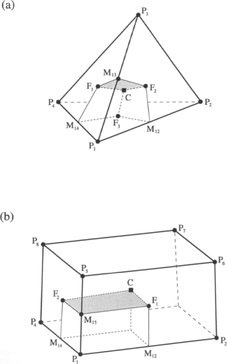
图5.7:四面体(a)与六面体(b)的中位对偶格式的部分控制体及面(阴影所示)。P表示网格节点,C为单元形心(方程(5.17)),F为面形心(方程(5.8)或(5.9)),M表示边中点。阴影部分表示分配给边\(P_1-P_3\)或\(P_1-P_5\)的控制体面的一部分。
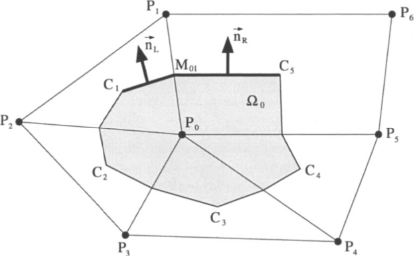
图5.8:中位对偶格式的控制体(二维)。\(C_1\)、\(C_2\)等表示单元中心(形心);\(P_1\)、\(P_2\)等表示网格节点。与边\(P_0-P_1\)相关联的面面积用粗线标出。图中还标出了部分面的单位法向量\(\vec{n}_L\)、\(\vec{n}_R\)ï¼边\(P_0-P_1\)的中点\(M_{01}\)ï¼以及网格节点\(P_0\)周围的控制体\(\Omega_0\)。
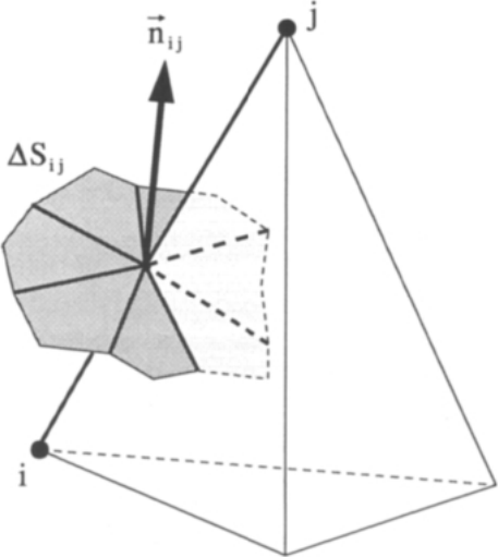
图5.9:三维中位对偶单元顶点格式中与边\(ij\)相关联的总面面积\(\Delta S_{ij}\)与平均单位法向量\(\vec{n}_{ij}\)。
通量的计算在形式上与单元中心格式所用的方法相同ï¼因此公式(5.18)-(5.22)在中位对偶格式中同样适用。如果采用上面这种把每条边与一个平均单位法向量相关联的做法ï¼那么最有效率的方法是在空间离散化中采用基于边(edge-based)的数据结构。这种数据结构对网格中每条具体的边(参见图5.9)存储:
- 指向定义该边的两个节点的指针——借此可以访问与两个控制体\(\Omega_i\)和\(\Omega_j\)相关联的流动变量;
- 面向量(\(\vec{S}_{ij} = \vec{n}_{ij}\Delta S_{ij}\))——必须一致地指向外侧或内侧;
- 从节点\(i\)指向节点\(j\)的边向量——把流动变量插值到面上(解的重构)时需要。另一种做法是ï¼边向量可以由节点坐标即时算得。对于带人工耗散的标准中心格式(5.3.1小节)ï¼此项并不需要。
en
The computation of fluxes follows formally the same approaches as for the cell-centred scheme. Thus, the formulae (5.18)-(5.22) are applicable also in the case of the median-dual scheme. If we utilise the above approach which associates each edge with a mean unit normal, the most efficient methodology is to employ an edge-based data structure for the spatial discretisation. The edge-based data structure stores for each particular edge in the grid (cf. Fig. 5.9):
- pointers to the two nodes which define the edge - this allows us to access the flow variables associated with the two control volumes \(\Omega_i\) and \(\Omega_j\);
- the face vector (\(\vec{S}_{ij} = \vec{n}_{ij}\Delta S_{ij}\)) - must point consistently either outwards or inwards;
- the edge vector from node \(i\) to node \(j\) - required for the interpolation of flow variables to the face (solution reconstruction). Alternatively, the edge vector can be computed on the fly from coordinates of the nodes. This is not required for the standard central scheme with artificial dissipation (Subsection 5.3.1).
DO edge = 1, nedges
    i = pointer_to_left_node( edge )
    j = pointer_to_right_node( edge )
    (F dS)_ij = F(W_ij, n_ij) dS_ij   (approx.)
    R_i = R_i + (F dS)_ij
    R_j = R_j - (F dS)_ij
ENDDO
循环结束后ï¼再加上源项\(\vec{Q}_i\Omega_i\)ï¼就得到所有节点处的最终残差(\(\vec{R}\))。与对每个控制体分别累加通量相比ï¼这一方法的效率显著更高ï¼因为每个平均面向量只存储一次ï¼而且每条边也只访问一次而不是两次。此外ï¼由于我们使用完全相同的平均面向量\(\vec{S}_{ij}\)来计算流入体积\(\Omega_i\)和\(\Omega_j\)的部分通量ï¼质量、动量和能量严格保持守恒。en
After the loop is completed and the source term \(\vec{Q}_i\Omega_i\) is added, we obtain the final residuals (\(\vec{R}\)) in all nodes. This approach is significantly more efficient than summing up the fluxes over each control volume separately, because we store each mean face vector only once and we also visit each edge only once instead of twice. Furthermore, since we use exactly the same mean face vector \(\vec{S}_{ij}\) in order to to evaluate the partial fluxes into the volumes \(\Omega_i\) and \(\Omega_j\), the mass, momentum and energy remain exactly conserved.
5.2.3 Cell-Centred versus Median-Dual Scheme 单元中心格式与中位对偶格式的比较[cfd-5-2-3]
单元中心格式与中位对偶格式孰优孰劣ï¼一直是颇具争议的话题。主要原因在于ï¼缺少针对真实外形、在精度、计算时间和内存等方面对两种方法的公平比较。我们此处的意图ï¼是围绕以下四个方面收集支持与反对每种方法的最重要论据:
- 精度;
- 计算量;
- 内存需求;
- 灵活性。
en
The relative advantages and disadvantages of the cell-centred and the median-dual scheme are the subject of controversial debates. The main reason is the lack of fair comparisons of the two methodologies with respect to accuracy, computational time and memory for realistic configurations. Our intention here is to collect the most important arguments for and against each of the approaches regarding:
- accuracy,
- computational work,
- memory requirements, and
- flexibility.
这应有助于更深入地理解每种格式固有的问题ï¼并有助于针对具体的应用选择最合适的格式。en
This should lead to a greater understanding of the problems inherent to each scheme and should be of help in selecting the most suitable scheme for the intended applications.
Accuracy 精度
在三角形/四面体网格上ï¼单元中心格式得到的控制体数量(从而自由度)约为中位对偶格式的两倍/六倍[36]。在由四面体和棱柱构成的典型混合网格上ï¼单元中心格式给出的未知量数目约为中位对偶格式的三倍。这表明在相同网格上ï¼单元中心格式比单元顶点离散化更精确。然而ï¼与中位对偶格式相比ï¼单元中心格式的残差由少得多的通量累加而成(在四面体网格上约为三个对七个)ï¼这可能损害精度。因此ï¼究竟哪种格式更优ï¼并没有明确的证据。en
A cell-centred scheme on a triangular/tetrahedral grid leads to about twice/six times as many control volumes and hence degrees of freedom as a median-dual scheme [36]. On typical mixed grids, which consist of tetrahedra and prisms, a cell-centred scheme gives roughly three times more unknowns than a median-dual scheme. This suggests that cell-centred schemes are more accurate than cell-vertex discretisations on an identical grid. However, the residual of a cell-centred scheme results from a much smaller number of fluxes as compared to a median-dual scheme (three versus approximately seven on a tetrahedral grid), which may impair the accuracy. Thus, there is no clear evidence about which scheme might be superior.
中位对偶格式在拉伸的三角形和四面体网格上存在一个特有的问题。例如考虑图5.10ï¼它显示了由直角三角形组成的网格剖分ï¼这种剖分常用于黏性流动中的固体壁面附近。从图5.10a可以看到ï¼面\(\Delta S_{ij}\)相对于边\(ij\)变得高度倾斜。然而ï¼空间离散格式大多假设通量与面正交(尤其是黎曼求解器)。由此引入的误差对一阶格式尤为显著[38]。采用所谓的包含对偶(containment-dual)控制体[39]可以改善这一状况。如图5.11所示ï¼包含对偶方法用最小外包圆/球的中心代替单元形心来定义面。这样得到的控制体与四边形网格上的相同(图5.10b)。注意ï¼像\(ij'\)这样的对角边没有与之相关联的面面积。这需要额外的预处理工作量ï¼但解的精度可以得到明显改善[40]。当然ï¼另一种可能的做法是直接在(边界层内)采用四边形或六面体en
The median-dual scheme suffers from a particular problem on stretched triangular and tetrahedral grids. Consider, for example, Fig. 5.10, which shows a tessellation composed of right triangles, as it is often employed near solid walls for viscous flows. We can see in Fig. 5.10a that the face \(\Delta S_{ij}\) becomes highly skewed with respect to the edge \(ij\). However, spatial discretisation schemes mostly assume fluxes to be orthogonal to a face (especially Riemann solvers). Thus, an error is introduced which is particularly significant for a first-order scheme [38]. The situation can be improved using the so-called containment-dual control volume [39]. As depicted in Fig. 5.11, the containment-dual approach employs the centres of the minimum spanning circles/spheres instead of the cell centroids to define the faces. This leads to control volumes identical to those on quadrilateral grids (Fig. 5.10b). Notice that there is no face area associated with diagonal edges like \(ij'\). An additional effort is required for pre-processing, but the solution accuracy can be improved noticeably [40]. Of course, another possibility is to employ directly quadrilateral or hexahedral
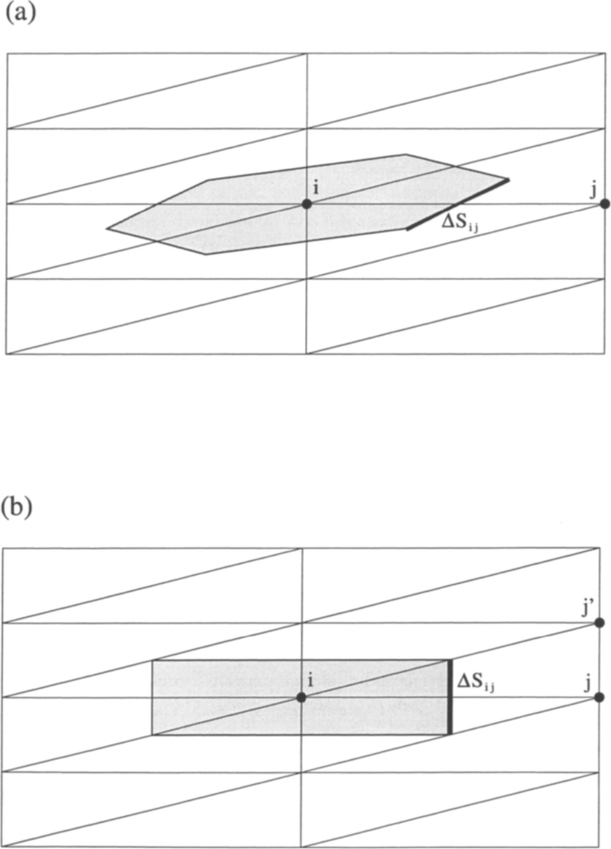
图5.10:对拉伸直角三角形剖分ï¼中位对偶(a)与包含对偶(b)控制体的比较。图例:阴影部分为控制体,\(i\)、\(j\)为节点,\(\Delta S_{ij}\)为与边\(ij\)相关联的(粗线所示)面;(b)中\(j'\)为包含对偶在最长边上引入的节点。
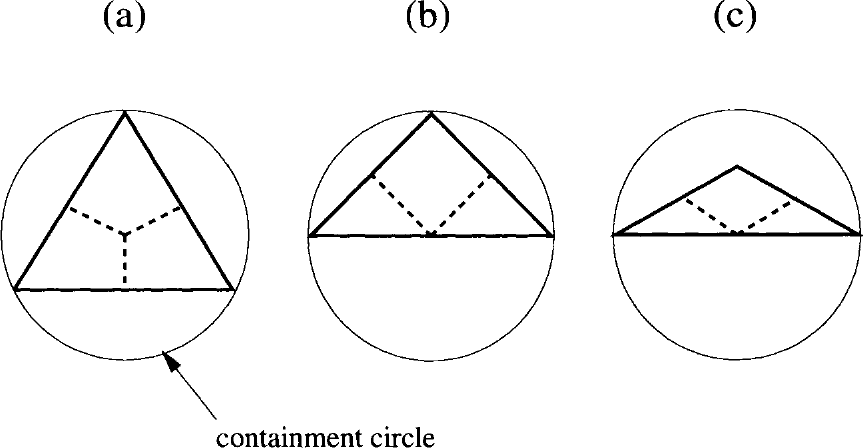
图5.11:锐角(a)与钝角(c)三角形情形下包含对偶(虚线)的一部分[40]。包含圆(containment circle)是包含该三角形的最小圆;对钝角三角形ï¼它的圆心位于最长边上。
(单元)。关于网格诱导误差的进一步讨论可参见文献[22]和[23]。en
cells within the boundary layers. Further discussion of grid-induced errors can be found in Ref. [22] and [23].
中位对偶格式固有的另一个问题ï¼出现在物理域边界处的离散化。具体而言ï¼在边界处只剩下大约半个控制体(参见图4.6)。围绕各面对通量积分ï¼得到的残差位于控制体内部(inside)——理想情况下在其中心(centre);然而ï¼残差却被关联到直接位于边界上的节点(node)。与单元中心格式相比ï¼这种失配导致离散化误差增大ï¼这在固体壁面上尤其不利。对偶控制体的定义还会在尖锐角点(如尾缘)处引起问题ï¼表现为压力或密度中的非物理峰值。在周期性边界处(参见第8.8章)还会出现进一步的复杂情况:必须把来自控制体两部分的通量正确地相加。en
Another problem inherent to the median-dual scheme is the discretisation at boundaries of the physical domain. What happens is that there is only about one half of the control volume left at the boundary (cf. Fig. 4.6). The integration of fluxes around the faces results in a residual located inside - ideally at the centre - of the control volume. However, the residual is associated with the node, residing directly on the boundary. This mismatch leads to increased discretisation error in comparison to the cell-centred scheme, which is particularly undesirable on solid walls. The definition of the dual control volume causes also problems at sharp corners (like trailing edges), which show up as unphysical peaks in pressure or density. Further complications arise at periodic boundaries (see Chapter 8.8), where the fluxes from both parts of the control volume have to be summed up correctly.
控制体形心与残差存储节点之间的失配ï¼对中位对偶格式还有进一步的影响:在非定常流动情形下ï¼它表现为质量矩阵。这一点我们在3.2节开头已经讨论过。单元中心格式的优点是ï¼可以在不牺牲解的精度的情况下从方程中消去质量矩阵;与此相反ï¼中位对偶格式需要对质量矩阵作特殊处理[41]、[42]。en
The mismatch between the centroid of the control volume and the node where the residual is stored has also a further implication for the median-dual scheme. It arises as the mass matrix in the case of unsteady flows. We discussed this point already at the beginning of Section 3.2. The advantage of the cell-centred scheme is that the mass matrix can be eliminated from the equations, without compromising the solution accuracy. By contrast, the median-dual scheme requires a special treatment of the mass matrix [41], [42].
Computational Work 计算量
要判断两种格式所需的计算量ï¼主要须考察通量的积分。从前面的讨论可知ï¼单元中心格式对单元面作循环ï¼而中位对偶格式对边作循环。由于两种格式在交界面上计算通量的方式相当类似ï¼单元面数与边数之比就给出了计算量之比。因此ï¼在四面体网格上ï¼单元面数(若每两个单元只计一次)约为边数的两倍ï¼因而在相同网格上ï¼单元中心格式的计算代价约为中位对偶格式的两倍[36]。然而ï¼在含棱柱单元的混合网格上ï¼单元中心方法变得更有竞争力。在六面体网格上ï¼面数等于边数ï¼除边界处理外ï¼两种方法的计算量相当。en
In order to judge the computational effort required for both schemes, we have to consider primarily the integration of the fluxes. We know from the previous discussion that the cell-centred scheme uses a loop over cell faces whereas the median-dual scheme loops over the edges. Since the evaluation of the fluxes at an interface is quite similar for both schemes, the ratio of the number of cell faces to the number of edges gives the ratio of the computational work. Thus, on a tetrahedral grid, where the number cell faces (if counted only once for every two cells) is approximately two times larger than the number of edges, the cell-centred scheme is computationally twice as much expensive as the median-dual scheme on an identical grid [36]. The cell-centred approach becomes however more competitive on mixed grids containing prismatic elements. Apart from boundary treatment, both methods are computationally equivalent on hexahedral grids, where the number of faces equals the number of edges.
Memory Requirements 内存需求
就内存需求而言ï¼与中位对偶格式相比ï¼单元中心格式在四面体网格上需要存储的流动变量约为其六倍ï¼在通常的混合网格上约为其三倍。此外ï¼如前所述ï¼两种格式都需要为每个单元面或每条边分别存储两个整数和三个实数(指针与面向量)。另外ï¼单元中心格式还必须在内存中为每个单元面保存两个指向面中点的向量——6个实数。相反ï¼中位对偶格式只依靠节点坐标即可工作ï¼所需数值要少得多。总而言之ï¼平均来说ï¼单元中心格式所需的计算机内存是中位对偶方法的两倍以上。en
Considering the memory requirements, the cell-centred scheme has to store about six times more flow variables on tetrahedral and about three times more variables on usual mixed grids as compared to the median-dual scheme. Furthermore, as we saw, both schemes require to store two integers and three reals (pointers and face vector) per cell face or edge, respectively. Additionally, the cell-centred scheme has to keep two vectors to the face-midpoint - 6 reals - per cell face in memory. On the contrary, the median-dual scheme can work with the node coordinates only, which are considerably fewer values. Thus in summary, the cell-centred scheme needs, on average, more than twice as much computer memory as the median-dual method.
Grid Generation/Adaptation 网格生成/自适应
单元中心格式的一个显著优势出现在非相容(non-conforming)单元界面的情形ï¼例如图3.4中字母“F”处的界面。与中位对偶方法不同ï¼在这种界面上计算通量不需要特殊而昂贵的处理。这使网格生成和网格自适应的灵活性得以提高。en
One significant advantage of the cell-centred scheme appears in the case of non-conforming cell interfaces, like those at the letter "F" in Fig. 3.4. In contrast to the median-dual methodology, no special and expensive procedure is required for the computation of the fluxes at the interface. This allows for an increased flexibility in the grid generation and also in the grid adaptation.
5.3 Discretisation of the Convective Fluxes 对流通量的离散[cfd-5-3]
在前面几节中ï¼我们讨论了各种可能的空间离散方法学的一般性问题ï¼包括必要的数据结构。接下来ï¼我们将更深入地了解对流通量的计算究竟如何实现。en
In the previous sections, we considered general issues of possible spatial discretisation methodologies including the necessary data structures. In what follows, we shall learn more about the details, how the evaluation of the convective fluxes can be implemented.
正如我们在3.1.5小节中已经看到的ï¼在有限体积方法的框架内ï¼基本上可以在以下几类格式之间选择:
- 中心格式;
- 通量向量分裂;
- 通量差分分裂;
- 总变差减小(TVD);以及
- 脉动分裂(fluctuation-splitting)
en
As we could already see in Subsection 3.1.5, in the framework of the finite volume approach, we have basically the choice between:
- central,
- flux-vector splitting,
- flux-difference splitting,
- total variation diminishing (TVD), and
- fluctuation-splitting
……格式。首先ï¼我们将较为详细地介绍非结构网格上的中心离散ï¼因为它与结构网格上的做法差别很大。相反ï¼上风格式的基本原理在结构网格与非结构网格上是相同的ï¼因此其细节可参见4.3.2-4.3.4节。然而ï¼非结构网格上的新内容是解重构(solution reconstruction)ï¼即为了得到控制体面上的流动变量值所必需的步骤。因此ï¼我们将在5.3.3小节中较为详细地讨论各种常用方法。限于篇幅ï¼这里不讨论仍处于研究状态的脉动分裂方法。与脉动分裂格式相关的文献ï¼读者可参阅3.1.5小节。en
schemes. First of all, we shall present the central discretisation on unstructured grids at some length, since it differs considerably from that on structured grids. On the contrary, the basics of the upwind schemes are identical on structured and unstructured grids. Hence, the details can be found in Sections 4.3.2-4.3.4. However, what is new on unstructured grids is the solution reconstruction, which is required in order to obtain the values of the flow variables at a face of the control volume. Therefore, we shall discuss the common approaches in some detail in Subsection 5.3.3. Because of space limitations, we will not treat the fluctuation-splitting approach here, which is still in research status. The reader is referred to Subsection 3.1.5 for the bibliography related to fluctuation-splitting schemes.
5.3.1 Central Schemes with Artificial Dissipation 带人工耗散的中心格式[cfd-5-3-1]
中心格式的基本思想ï¼是按照方程(5.20)ï¼用控制体面两侧守恒变量的算术平均来计算该面上的对流通量。这会导致解的奇偶失联(odd-even decouplingï¼即离散方程产生两个相互独立的解)以及激波处的波动ï¼因此为了保持稳定性必须加入人工耗散。人工耗散基于二阶与四阶差分的混合。该格式由Jameson等人[43]最先在结构网格上针对欧拉方程实现。以各位作者姓氏的首字母命名ï¼它也简称为JST格式。en
The basic idea of the central scheme is to compute the convective fluxes at a face of the control volume from the arithmetic average of the conservative variables on both sides of the face according to Eq. (5.20). Since this would lead to odd-even decoupling of the solution (generation of two independent solutions of the discretised equations) and wiggles at shocks, artificial dissipation has to be added for stability. The artificial dissipation is based on a blend of second- and fourth-order differences. The scheme was first implemented for the Euler equations on structured grids by Jameson et al. [43]. Because of the names of the authors, it is also abbreviated as the JST scheme.
在非结构网格上实现JST格式时ï¼二阶差分采用拉普拉斯(Laplacian)算子ï¼四阶差分采用拉普拉斯的拉普拉斯[44]、[27]。为了降低计算成本ï¼采用伪拉普拉斯算子(pseudo-Laplacian)代替真正的拉普拉斯算子。为此,[45]首先提出了二维格式ï¼随后[46]作了改进。后来,[2]把该格式推广到三维。它利用了一种距离加权过程。这样ï¼对于任何网格上线性变化的函数ï¼该格式的伪拉普拉斯算子都为零。应用于单元\(I\)中的某一般标量\(U\)时ï¼伪拉普拉斯算子的形式为en
The implementation of the JST scheme on unstructured grids utilises the Laplacian operator for the second-order differences and the Laplacian of Laplacian for the fourth-order differences [44], [27]. In order to reduce the computational cost, pseudo-Laplacians are employed instead of true Laplacians. For this purpose, a 2-D formulation was proposed first in [45] and then improved in [46]. Later on, the scheme was extended to 3D in [2]. It makes use of a distance-weighting procedure. In this way, the scheme leads to a vanishing pseudo-Laplacian for a linearly varying function on any grid. Applied to a general scalar quantity \(U\) in cell \(I\), the pseudo-Laplacian assumes the form
其中\(N_A\)表示相邻控制体的数目。在采用中点对偶格式(median-dual scheme)时ï¼单元指标须换成节点指标\((i,j)\)。式(5.24)中的求和最好像通量计算那样ï¼用对面(单元中心格式)或对边(中点对偶格式)的循环来计算。几何权重\(\theta\)定义为en
where \(N_A\) stands for the number of adjacent control volumes. The cell indices have to be substituted by node indices \((i,j)\) in the case of the median-dual scheme. The sum in Eq. (5.24) is best evaluated using either a loop over faces (cell-centred scheme) or a loop over edges (median-dual scheme) similar to the flux computation. The geometrical weights \(\theta\) are defined as
权重由一个优化问题的解得到[2]。该优化问题借助拉格朗日乘子求解。由此ï¼几何权重由下式给出en
and result from the solution of an optimisation problem [2]. The optimisation problem is solved by means of Lagrange multipliers. Herewith, the geometrical weights are obtained from the expression
其中\(x\)、\(y\)、\(z\)为单元形心的笛卡尔坐标(中点对偶格式则为节点坐标)。拉格朗日乘子\(\lambda\)对每个单元(节点)计算ï¼由[2]得en
where \(x,y,z\) are the Cartesian coordinates of the cell centroids (nodes in the case of the median-dual scheme). The Lagrange multipliers \(\lambda\) are computed for each cell (node) and follow from [2]
其中的系数为en
with the coefficients
对单元\(I\)写出ï¼一阶矩为en
Written for a cell \(I\), the first-order moments read
此外ï¼二阶矩由下式给出en
Furthermore, the second-order moments are given by
几何权重(5.25)在严重扭曲的网格上可能导致拉普拉斯算子的非正近似ï¼从而使稳定性丧失。因此,[45]建议把权重限制在\((0,2)\)范围内。不过ï¼这一措施会损害离散的精度。更多细节另见文献[12]中的讨论。en
The geometrical weights (5.25) can lead to a non-positive approximation of the Laplacian and hence to a lost of stability on severely distorted grids. Therefore, clipping the weights to the range \((0,2)\) was suggested in [45]. However, this measure impairs the accuracy of the discretisation. See also the discussion in Ref. [12] for further details.
其中\(N_F\)表示控制体的面数(它可能与相邻控制体的数目不同ï¼例如当一个四边形面被分成两个三角形时)。en
where \(N_F\) denotes the number of the faces of the control volume (which may differ from the number of adjacent control volumes, e.g., if a quadrilateral face is divided into two triangles).
其中\(V_m\)表示逆变速度(2.22),\(c_m\)为声速。这两个量都用面上平均的流动变量计算。控制体面上的谱半径由下式得到en
where \(V_m\) represents the contravariant velocity (2.22) and \(c_m\) the speed of sound, respectively. Both quantities are computed from flow variables averaged at the face. The spectral radius at the face of the control volume is obtained from
利用一个基于压力的传感器ï¼在激波处关闭四阶差分ï¼在流场的光滑区域关闭二阶差分。据此ï¼式(5.31)中的系数\(\epsilon_{IJ}^{(2)}\)与\(\epsilon_{IJ}^{(4)}\)定义为en
A pressure-based sensor is used to switch off the fourth-order differences at shocks and the second-order differences in smooth portions of the flow field. Herewith, the coefficients \(\epsilon_{IJ}^{(2)}\) and \(\epsilon_{IJ}^{(4)}\) in Eq. (5.31) are defined as
其中的压力传感器由下式给出en
with the pressure sensor given by
参数的典型取值为\(k^{(2)} = 1/2\)ï¼以及\(1/128 \le k^{(4)} \le 1/64\)。en
Typical values of the parameters are \(k^{(2)} = 1/2\) and \(1/128 \le k^{(4)} \le 1/64\).
正如我们在4.3.1小节中已经讨论过的ï¼若在式(5.31)中用一个矩阵[47]代替谱半径\((\hat{\Lambda}_c)_{IJ}\)ï¼上述中心格式的精度可以得到改进。这种所谓的矩阵耗散(matrix dissipation)格式在非结构网格上的实现方式与结构网格相同ï¼缩放矩阵的定义如同式(4.59)。矩阵耗散格式在三维混合网格上的应用可参见例如文献[48]。en
As we already discussed in Subsection 4.3.1, the accuracy of the above central scheme can be improved when we substitute a matrix [47] for the spectral radius \((\hat{\Lambda}_c)_{IJ}\) in Eq. (5.31). The implementation of this so-called matrix dissipation scheme on unstructured grids proceeds in the same way as on structured grids, with the scaling matrix defined as in Eq. (4.59). Application of the matrix dissipation scheme to 3-D mixed grids is discussed, e.g., in Ref. [48].
需要特别注意的是ï¼对于三角形/四面体以外的单元ï¼常用的显式Runge-Kutta型时间离散在与中心格式耦合时会出现严重的稳定性问题[49]。原因在于四阶差分是用拉普拉斯的拉普拉斯来表示的。一种补救办法是用左、右状态之差(参见4.3节)来近似四阶差分[49]ï¼即en
It is important to note that for elements other than triangles/tetrahedra, the popular explicit Runge-Kutta type of temporal discretisation experiences severe stability problems when it is coupled to the central scheme [49]. The reason is the representation of the fourth-order differences by the Laplacian of the Laplacian. A remedy is to employ a difference of the left and the right state (cf. Section 4.3) for the approximation of the fourth-order differences [49], i.e.,
这种做法在四边形/六面体网格上给出与相应结构格式相同的模板。左、右状态可用例如下文5.3.3小节所述的线性重构来计算。en
This approach leads on quadrilateral/hexahedral grids to the same stencil as the corresponding structured scheme. The left and right state are computed using, e.g., the linear reconstruction described below in Subsection 5.3.3.
5.3.2 Upwind Schemes 上风格式[cfd-5-3-2]
至少就目前而言ï¼上风格式在非结构网格上似乎比上述中心格式更受欢迎。实际上,Roe的通量差分分裂格式[50]是非结构网格上应用最广的方法。与中心格式相比ï¼它对边界层的分辨率明显更高ï¼对网格扭曲的敏感性更低ï¼这正是Roe格式吸引人的地方。然而ï¼性能改善的代价是更大的计算量——当必须使用限制器来抑制解的振荡时(5.3.5小节)ï¼这一代价变得相当可观。en
Upwind schemes seem to have gained, at least for the moment, much more popularity on unstructured grids than the above central scheme. In fact, the flux-difference splitting scheme of Roe [50] is the most widely employed approach on unstructured grids. It is the considerably more accurate resolution of boundary layers and the lower sensitivity to grid distortions in comparison to the central scheme, which explains the attractiveness of Roe's scheme. However, the price to be paid for the improved performance is the higher computational effort, which becomes quite significant if a limiter has to be used to suppress oscillations of the solution (Subsection 5.3.5).
4.3节中针对结构网格介绍的各种上风格式ï¼无需改动基本方法学即可用于非结构网格。只有左、右状态的计算(式(5.22))——即所谓的解重构——以及限制函数的计算需要新的公式。因此ï¼这里只讨论解重构与限制器。关于各种上风方法的细节ï¼读者可参阅4.3.2-4.3.4小节。采用中点对偶方法在非结构网格上实现Roe格式的例子可参见例如文献[33]。en
Any of the upwind schemes presented in Section 4.3 for structured grids are applicable to unstructured grids without modifications to the basic methodology. Only the computation of the left and right state (Eq. (5.22)), which is denoted as solution reconstruction, as well as the evaluation of the limiting function require new formulations. For this reason, only the solution reconstruction and the limiters are discussed here. For details on the various upwind methods, the reader is referred to Subsections 4.3.2-4.3.4. An example for the implementation of Roe's scheme on unstructured grids using the median-dual approach can be found, e.g., in Ref. [33].
5.3.3 Solution Reconstruction 解重构[cfd-5-3-3]
正如我们在4.3.2-4.3.4小节中所看到的ï¼上风格式要求在控制体面的左、右两侧给定流动状态。式(5.37)中改进的人工耗散格式也是如此。en
As we saw in Subsections 4.3.2-4.3.4, upwind schemes require flow states to be specified on the left and the right side of a control volume face. The same holds also for the modified artificial dissipation scheme in Eq. (5.37).
作为第一种做法ï¼可以假设解在每个控制体内部为常数。此时左、右状态就是为左、右控制体计算的流动变量。例如ï¼对中点对偶格式(图5.9)ï¼我们会取en
As a first approach, we can assume that the solution is constant inside each control volume. The left and right state are then simply the flow variables computed for the left and the right control volume. For example, in the case of the median-dual scheme (Fig. 5.9) we would set
其中\(U\)代表某个标量流动变量。这样得到的空间离散只有一阶精度。对黏性流动而言ï¼一阶精度的解耗散太大ï¼会导致剪切层过度增长。因此ï¼计算黏性流动必须采用空间精度更高的方法。en
with \(U\) representing some scalar flow variable. This leads to a spatial discretisation which is only first-order accurate. For viscous flows, a first-order accurate solution is too diffusive and leads to an excessive growth of shear layers. Therefore, methods with higher spatial accuracy are a must for the computation of viscous flows.
如果假设解在控制体内部有变化ï¼就可以达到二阶及更高阶精度。二阶精度方法是最常用的高阶方法ï¼它假设解在控制体上按线性方式变化。为了计算左、右状态ï¼需要对所假设的解的变化进行重构。下面我们将讨论线性变化与二次变化重构的最常用方法。关于各种线性重构技术的比较ï¼有兴趣的读者可参阅[38]。en
We can achieve second- and higher-order accuracy if we assume the solution changes over the control volume. For second-order accurate methods, which are the most commonly employed higher-order methods, the solution is assumed to vary in a linear fashion over the control volume. In order to compute the left and right state, a reconstruction of the assumed solution variation becomes necessary. In what follows, we shall discuss the most popular approaches for the reconstruction of linear and quadratic variations. The interested reader is referred to [38] for a comparison of various linear reconstruction techniques.
Reconstruction Based on MUSCL Approach 基于MUSCL方法的重构
达到二阶精度的一种可能途径ï¼是把MUSCL方法[51]推广到非结构网格。当用于中点对偶格式时ï¼该方法为每条边\(ij\)生成两个“虚拟”节点\(i'\)与\(j'\)[52]-[56]。如图5.12所示ï¼这些虚拟节点位于把边\(ij\)向两端各延长一个边长所得线段的端点处。在把解从周围单元(图5.12中着灰色者)插值到虚拟节点之后ï¼便可用MUSCL公式即式(4.46)计算左、右状态。于是,en
One possibility to achieve second-order accuracy consists of the extension of the MUSCL approach [51] to unstructured grids. When applied to the median-dual scheme, the method generates for each edge \(ij\) two "phantom" nodes \(i'\) and \(j'\) [52]-[56]. These phantom nodes are located at the endpoints of the line obtained by extending the edge \(ij\) by its length in both directions as sketched in Fig. 5.12. After the solution is interpolated from the surrounding elements (gray coloured in Fig. 5.12) to the phantom nodes, we can evaluate the left and right state using the MUSCL formulae Eq. (4.46). Hence,
其中前向\((\Delta_{+})\)与后向\((\Delta_{-})\)差分算子定义为en
with forward \((\Delta_{+})\) and the backward \((\Delta_{-})\) difference operators defined as
出现强间断时,MUSCL插值(5.39)必须辅以限制器函数(按照4.3.5小节)。这种方法的一个缺点是必须为每条边存储包含虚拟节点的单元。另一个概念上的缺点是:为一个控制体重构出的梯度并不唯一。此外ï¼在边界处可能出现困难ï¼因为此时某个虚拟点会落在物理域之外。en
The MUSCL interpolation (5.39) has to be enhanced by a limiter function (according to Subsection 4.3.5) in the case of strong discontinuities. A disadvantage of this methodology is the necessity to store for each edge the elements which contain the phantom nodes. A further conceptual disadvantage is that no unique gradient is reconstructed for a control volume. Furthermore, difficulties can arise at boundaries, where one of the phantom points lies outside the physical domain.
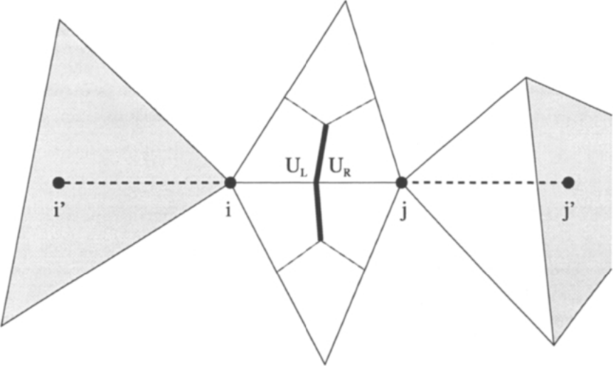
图5.12:基于沿边ij方向的单元插值确定左、右状态(二维中点对偶格式)。图例:\(i'\)、\(i\)、\(j\)、\(j'\)——虚拟节点与边ij的端点;\(U_L\)、\(U_R\)——控制体面上的左状态与右状态;着灰色的单元表示用于插值到虚拟节点的周围单元;虚线表示由边ij向两端延长所得的线段。
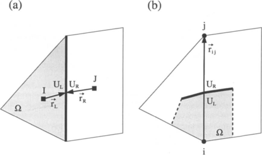
图5.13:二维单元中心格式(a)与中点对偶格式(b)的线性重构。图例:(a)\(I\)、\(J\)——单元形心;\(U_L\)、\(U_R\)——面上的左、右状态;\(\vec{r}_L\)、\(\vec{r}_R\)——由形心指向面中点的向量;\(\Omega\)——控制体。(b)\(i\)、\(j\)——节点;\(\vec{r}_{ij}\)——由节点\(i\)指向\(j\)的边向量;\(U_L\)、\(U_R\)——面上的左、右状态;\(\Omega\)——对偶控制体。
Piecewise Linear Reconstruction 分段线性重构
Barth与Jespersen在[30]中提出了一种与有限元格式密切相关的重构方法。这里假设解在控制体上分段线性分布。于是ï¼对单元中心格式ï¼可由下列关系式求出左、右状态en
Barth and Jespersen presented in [30] a reconstruction method, which is closely related to the finite element schemes. Here, it is assumed that the solution is piecewise linearly distributed over the control volume. Then, we can find the left and right state for a cell-centred scheme from the relations
其中\(\nabla U_I\)是\(U\)(即\([\partial U/\partial x,\, \partial U/\partial y,\, \partial U/\partial z]^T\))在单元中心\(I\)处的梯度,\(\Psi\)表示限制器函数(参见5.3.5小节)。向量\(\vec{r}_L\)与\(\vec{r}_R\)从单元形心指向面中点ï¼如图5.13a所示。en
where \(\nabla U_I\) is the gradient of \(U\) (\(= [\partial U/\partial x,\, \partial U/\partial y,\, \partial U/\partial z]^T\)) at the cell centre \(I\) and \(\Psi\) denotes a limiter function (cf. Subsection 5.3.5), respectively. The vectors \(\vec{r}_L\) and \(\vec{r}_R\) point from the cell-centroid to the face-midpoint, as indicated in Fig. 5.13a.
同样的方法也适用于中点对偶格式[30]ï¼即en
The same approach applies to the median-dual scheme [30], i.e.,
按照图5.9或图5.13b,en
According to Fig. 5.9 or Fig. 5.13b,
表示从节点\(i\)指向节点\(j\)的向量。en
represents the vector from node \(i\) to node \(j\).
容易看出,Barth与Jespersen的方法相当于围绕面相邻的形心/节点作泰勒级数展开并只保留线性项。线性重构在规则网格上形式上为二阶精度[38]。只要梯度\(\nabla U\)的计算没有误差ï¼该格式在任意网格上都能精确重构线性函数。线性重构很可能是各种重构方法中最常用的一种。en
It can be easily seen that the method of Barth and Jespersen corresponds to a Taylor-series expansion around the neighbouring centres/nodes of the face, where only the linear term is retained. The linear reconstruction is formally second-order accurate on regular grids [38]. The scheme reconstructs a linear function exactly on any grid, provided the gradient \(\nabla U\) is evaluated without an error. The linear reconstruction is likely the most popular one among the reconstruction methods.
上述格式需要在单元中心或节点处计算梯度。这既可以用Green-Gauss方法也可以用最小二乘方法实现ï¼二者将在下文5.3.4小节中介绍。此外ï¼限制器函数在非结构网格上的实现将在5.3.5小节中详细描述。en
The above scheme requires the computation of gradients at cell centres or at nodes, respectively. This can be accomplished either by the Green-Gauss or the least-squares approach, which are presented below in Subsection 5.3.4. Furthermore, the implementation of the limiter function on unstructured grids is described in detail in Subsection 5.3.5.
Linear Reconstruction Based on Nodal Weighting Procedure 基于节点加权过程的线性重构
Frink[26]证明ï¼对单元中心格式ï¼在纯三角形或四面体网格上线性重构(5.41)无需显式计算梯度。原因在于这类单元的两个不变几何特征。其一ï¼从任一节点出发穿过单元形心的直线总会与对面(与该节点相对的面)的中点相交。其二ï¼从单元形心到面中点的距离ï¼是从面中点到对面节点距离的四分之一(对三角形为三分之一)。这样ï¼单元中心处的梯度便可用简单有限差分近似[26]。例如ï¼若要重构图5.7a中面中点\(F_3\)处的解ï¼式(5.41)就成为en
It was demonstrated by Frink [26] that for the cell-centred scheme the linear reconstruction (5.41) does not require an explicit evaluation of the gradient on purely triangular or tetrahedral grids. The reason are two invariant geometric features of these elements. First, a line from a node through the cell-centroid will always intersect the midpoint of the opposing face. Second, the distance from the cell-centroid to the face-midpoint is one-fourth (one-third for a triangle) of the distance from the face-midpoint to the opposite node. Thus, the gradient at the cell centre can be approximated by a simple finite difference [26]. For example, if we were to reconstruct the solution at the face-midpoint \(F_3\) in Fig. 5.7a, the formulae (5.41) would become
其中\(U_C\)为单元形心处的值,\(U_1\)、\(U_2\)等表示节点值ï¼而\(\Psi\)表示限制器。en
with \(U_C\) being the value at the cell-centroid, \(U_1\), \(U_2\), etc. denoting the nodal values, and finally \(\Psi\) standing for a limiter, respectively.
Frink设计了两种确定节点值的方法。第一种基于逆距离加权(inverse distance weighting)。此时ï¼周围单元对某节点的贡献与该节点到单元形心的距离成反比[26]、[57]ï¼即en
Two different ways were devised by Frink in order to determine the nodal values. The first approach is based on inverse distance weighting. Here, the contribution to a node from the surrounding cells is inverse proportional to the distance from the node to the cell-centroid [26], [57], i.e.,
其中权重\(\theta_{iJ} = 1/r_{iJ}\)。距离按下式计算en
with the weights \(\theta_{iJ} = 1/r_{iJ}\). The distance is computed from
下标\(J\)与\(i\)分别指单元形心与节点。上述方法得到的重构不足二阶精度。不过Frink指出ï¼至少对无黏流动不需要限制器[26]ï¼从而显著减少了计算量。en
The subscripts \(J\) and \(i\) refer to the cell-centroid and to the node, respectively. The above methodology leads to a reconstruction which is less than second-order accurate. However, Frink pointed out that no limiter is needed at least for inviscid flows [26], which reduces the computational effort significantly.
第二种方法基于Holmes等人[45]与Rausch等人[46]在二维上的工作ï¼后来由Frink[2]推广到三维。这里ï¼式(5.45)中的权重\(\theta_{iJ}\)定义为:当变化为线性时ï¼节点值可被精确算出。这导致与伪拉普拉斯算子(5.24)的计算相同的约束条件ï¼因此权重也相同ï¼由式(5.25)-(5.30)给出ï¼只需把单元形心坐标\(x_I\)、\(y_I\)、\(z_I\)换成节点坐标\(x_i\)、\(y_i\)、\(z_i\)。由于节点值对线性函数是精确的ï¼该格式形式上为二阶精度。为了保证在扭曲网格上的正性ï¼权重必须限制在\((0,2)\)范围内[45]。遗憾的是ï¼这会降低重构的精度。Frink等人[4]最近还报道了该重构在Navier-Stokes方程下的一些异常行为。en
The second approach is based on work of Holmes et al. [45] and Rausch et al. [46] in 2D. It was later extended to 3D by Frink [2]. Here, the weights \(\theta_{iJ}\) in Eq. (5.45) are defined such that the nodal values are computed exactly if the variation is linear. This leads to the same constraints as for the computation of the pseudo Laplacian (5.24). Consequently, the weights are also the same and follow from the Equations (5.25)-(5.30). The coordinates \(x_I\), \(y_I\), \(z_I\) of the cell-centroids are just replaced by the node coordinates \(x_i\), \(y_i\), \(z_i\). The scheme is formally second-order accurate because the nodal values are computed exactly for a linear function. In order to assure positivity on distorted grids, the weights have to be restricted to the range \((0,2)\) [45]. Unfortunately, this reduces the accuracy of the reconstruction. Frink et al. [4] also recently reported some anomalous behaviour of the reconstruction for the Navier-Stokes equations.
Piecewise Quadratic Reconstruction 分段二次重构
要想用多项式重构达到高于二阶的精度ï¼就必须在围绕面相邻单元形心/节点的截断泰勒级数展开中保留更多项。基于Barth与Frederickson的工作[58],Barth提出了k精确(k-exact)重构格式的概念[59]ï¼即对\(k\)次多项式精确的重构。Barth方法中多项式的定义方式保证了均值守恒(conservation of the mean)ï¼换言之ï¼重构多项式的平均值等于控制体内的平均解。这一性质保证了重构过程中质量、动量与能量的守恒。该方法曾以\(k = 3\)在中点对偶格式中实现ï¼多项式系数用最小二乘方法计算。Mitchell与Walters[60]以及Mitchell[61]对单元中心格式遵循了类似思路。然而ï¼这些方法所需的数值工作量高得惊人ï¼数据结构也很复杂ï¼因而未能得到广泛应用。en
In order to achieve higher than second-order accuracy with a polynomial reconstruction, we have to keep further terms in the truncated Taylor-series expansion around the neighbouring cell-centres/nodes of the face. Based on the work of Barth and Frederickson [58], Barth developed the concept of k-exact reconstruction scheme [59], i.e., a reconstruction exact for a polynomial of degree \(k\). The polynomial in Barth's method is defined in a way which guarantees the conservation of the mean, or in other words, the average of the reconstruction polynomial is equal to the mean solution in the control volume. This property assures the conservation of mass, momentum, and energy during the reconstruction. The method was implemented for \(k = 3\) in a median-dual scheme. The coefficients of the polynomial were computed using a least-squares approach. Similar ideas were followed for the cell-centred scheme by Mitchell and Walters [60], and by Mitchell [61]. However, these methods require a prohibitively high numerical effort and a complex data structure which prevented their widespread use.
Delanaye与Essers[62]以及Delanaye[63]为单元中心格式发展了一种特殊的二次重构形式ï¼其计算效率高于Barth的方法。左、右状态用截断到二次项的泰勒级数近似[62]、[63]en
Delanaye and Essers [62] and Delanaye [63] developed a particular form of the quadratic reconstruction for cell-centred schemes, which is computationally more efficient than the method of Barth. The left and right state are approximated using Taylor series truncated after the quadratic term [62], [63]
该矩阵在单元形心\(I\)处取值。变量\(\Psi_{I,1}\)与\(\Psi_{I,2}\)分别表示用于线性项与二次项的两种不同限制器函数[62]。二次重构方法在规则网格上为三阶精度;由于误差项相消ï¼在任意网格上至少为二阶精度[63]。不过ï¼要达到这些性质ï¼必要条件是:式(5.47)中的梯度\(\nabla U\)至少以二阶精度计算,Hessian至少以一阶精度计算。这通过把Green-Gauss梯度计算与基于最小二乘的二阶导数近似相结合来实现[62]、[63]ï¼从而得到数值上高效的格式。但与线性重构相比ï¼其内存与CPU时间开销仍然相当可观。该方法使用由面相邻与节点相邻单元组成的固定模板。模板以及Green-Gauss梯度计算所用的积分路径示于图5.14。为了确定二次多项式的所有系数ï¼模板至少须提供六个(三维为十个)值。为了保持二次重构所提供的精度ï¼必须考虑解在面上的线性变化而不是常值。这意味着解必须在二维面的两个点——所谓Gauss求积点(参见图5.14)——处重构(三角面则为三个点)ï¼并且通量须在控制体面上分段积分[37]。en
evaluated at the cell-centroid \(I\). The variables \(\Psi_{I,1}\) and \(\Psi_{I,2}\) represent two different limiter functions for the linear and the quadratic term [62], respectively. The quadratic reconstruction method is third-order accurate on regular grids and at least second-order accurate on arbitrary grids due to cancellation of error terms [63]. Necessary conditions for achieving these properties are, however, that the gradient \(\nabla U\) in Eq. (5.47) is evaluated at least with second-order and the Hessian with first-order accuracy. This is accomplished by combining Green-Gauss gradient evaluation with least-squares based approximation of the second derivatives [62], [63], which leads to a numerically efficient scheme. But the memory and the CPU-time overheads are still quite significant in comparison to the linear reconstruction. The method utilises a fixed stencil composed of face and node neighbours. The stencil is shown in Fig. 5.14 together with the integration path employed for the Green-Gauss gradient computation. In order to determine all coefficients of the quadratic polynomial, at least six (ten in 3D) values must be provided by the stencil. To maintain the accuracy provided by the quadratic reconstruction, it is necessary to consider a linear variation of the solution over the face instead of a constant value. This implies that the solution must be reconstructed at two points - the so-called Gauss quadrature points (cf. Fig. 5.14) - of a 2-D face (at three points of a triangular face) and that the fluxes have to be integrated in a piecewise manner over the face of the control volume [37].
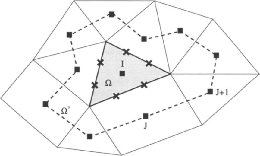
图5.14:Delanaye[62]、[63]二次重构方法在二维下的模板(实心矩形)。图例:虚线表示Green-Gauss梯度计算的积分路径(控制体\(\Omega'\));叉号表示通量积分的求积点;\(I\)、\(\Omega\)——中心单元及其控制体;\(J\)、\(J+1\)——模板中的远邻单元形心。
5.3.4 Evaluation of the Gradients 梯度的计算[cfd-5-3-4]
分段线性重构与二次重构的讨论中还遗留一个问题ï¼即梯度的确定。计算黏性通量(5.4节)也需要速度分量与温度的梯度。下面介绍两种方法:第一种基于Green-Gauss定理ï¼第二种利用最小二乘法。en
An open point, which remains from the discussion of the piecewise linear and the quadratic reconstruction, is the determination of the gradient. Gradients of the velocity components and the temperature are also required for the evaluation of the viscous fluxes (Section 5.4). Two approaches will be presented in the following: the first is based on the Green-Gauss theorem, and the second utilises the least-squares method.
Green-Gauss Approach Green-Gauss方法
该方法把某标量函数\(U\)的梯度近似为\(U\)与外指单位法向量的乘积在某个控制体\(\Omega'\)上的面积分ï¼即en
This method approximates the gradient of some scalar function \(U\) as the surface integral of the product of \(U\) with an outward-pointing unit normal vector over some control volume \(\Omega'\), i.e.,
Median-Dual Scheme 中点对偶格式
Barth与Jespersen[30]从Galerkin有限元方法导出了Green-Gauss方法的一种特殊离散。后来,Barth[64]把该离散推广到三维。Barth与Jespersen把式(5.49)应用于在某个节点处相会的所有单元的并集所构成的区域。他们证明ï¼这一方法可以表述成与基于边的数据结构相容的形式。不过ï¼这只对三角形/四面体网格上的中点对偶格式有效。所得公式为en
Barth and Jespersen [30] derived a particular discretisation of the Green-Gauss approach from the Galerkin finite element method. Later on, the discretisation was extended to 3D by Barth [64]. Barth and Jespersen applied Eq. (5.49) to the region formed by the union of the elements meeting at a node. They proved that the approach can be formulated such that it becomes compatible with the edge-based data structure. However, this works only for the median-dual scheme on triangular/tetrahedral grids. The resulting formula reads
这里ï¼式(5.49)中的\(\Omega'\)等于中点对偶控制体\(\Omega\)的体积。求和遍及与节点\(i\)相连的所有\(N_F\)条边。此外,\(\vec{n}_{ij}\)表示按式(5.23)定义的平均单位法向量,\(\Delta S_{ij}\)为总面面积。同一公式(5.50)在二维或三维都适用。需要指出的是ï¼为了得到一致的近似ï¼边界处的求和必须作改变[65](另见8.10节)。en
Here, \(\Omega'\) in Eq. (5.49) equals to the volume of the median-dual control volume \(\Omega\). The summation extends over all \(N_F\) edges incident to node \(i\). Furthermore, \(\vec{n}_{ij}\) denotes the average unit normal vector according to Eq. (5.23), and \(\Delta S_{ij}\) is the total face area, respectively. The same formula (5.50) is applicable in two or in three dimensions. It is important to mention that the summation has to be changed at boundaries in order to obtain a consistent approximation [65] (see also Section 8.10).
Cell-Centred Scheme 单元中心格式
Green-Gauss方法同样可用于单元中心格式。于是ï¼某单元形心\(I\)处的梯度可由下式得到en
We can use the Green-Gauss method in the cell-centred scheme as well. Hence, the gradient at some cell-centroid \(I\) can be obtained from
Mixed Grids 混合网格
用式(5.50)或式(5.51)计算Green-Gauss梯度的主要吸引力在于它与通量计算(如式(5.19))的相似性:这意味着梯度重构不需要额外的数据结构。主要缺点是式(5.50)或式(5.51)的近似在混合网格上会失效。[49]中证明ï¼梯度可能变得很不准确ï¼尤其是在不同单元类型相接之处。对中点对偶格式ï¼如果把式(5.49)中的体积\(\Omega'\)取为与节点\(i\)相关的所有单元的并集ï¼就可以解决这一问题。参照图5.8所示的情形ï¼二维梯度于是由下式给出en
The main attractiveness of the Green-Gauss gradient evaluation by Eq. (5.50) or (5.51) is its similarity to the computation of the fluxes (e.g., Eq. (5.19)). This means that no additional data structures are needed for the reconstruction of gradients. The main disadvantage is that the approximation in Eq. (5.50) or Eq. (5.51), respectively, fails on mixed grids. It was demonstrated in [49] that the gradient can become highly inaccurate, particularly where different element types meet. We can solve the problem in the case of the median-dual scheme when we keep the volume \(\Omega'\) in Eq. (5.49) identical to the union of all cells incident to node \(i\). Referring to the situation sketched in Fig. 5.8, the gradient results then in 2D from
其中取\(i = 0\)ï¼外表面数\(N_O = 6\)(由点\(P_1\)-\(P_6\)给出)ï¼当\(j = 6\)时\(j+1 = 1\)。此外,\(\vec{n}_j\)与\(\Delta S_j\)表示外单元面的单位法向量与面积。在三维中ï¼可用en
with \(i = 0\), the number of outer faces \(N_O = 6\) (given by the points \(P_1\)-\(P_6\)), and \(j+1 = 1\) for \(j = 6\). Furthermore, \(\vec{n}_j\) and \(\Delta S_j\) stand for the unit normal vector and the area of the outer cell faces. In 3D, we can use
这里假设所有的面都是三角形——或天然如此ï¼或经分解而成。同样的补救办法也可用于单元中心格式。此时控制体\(\Omega'\)的表面由远一与远二相邻单元的形心定义[62]、[63]ï¼如图5.14所示。梯度按式(5.52)或式(5.53)计算ï¼只是把节点指标换成单元指标。en
when we assume all faces are triangles - either naturally or by decomposition. The same remedy can be also employed for the cell-centred scheme. The surface of the control volume \(\Omega'\) is then defined by the centroids of the distant-one and distant-two neighbouring cells [62], [63], as it is rendered in Fig. 5.14. The gradient is computed correspondingly to Eq. (5.52) or (5.53) with cell instead of node indices.
这种基于单元的方法的明显缺点是必须增加一种数据结构ï¼以提供中心节点/形心与\(\Omega'\)外表面之间的联系。这样一来ï¼该方法不再是网格透明的(grid-transparentï¼即不再与单元信息无关)ï¼高效的gather-scatter循环也不再可能。这使得下面介绍的最小二乘技术在混合网格上更有吸引力。en
The clear disadvantage of such a cell-based approach is the necessity of an additional data structure, which provides a link between the central node/centroid and the outer faces of \(\Omega'\). Thus, the approach is no longer grid-transparent (i.e., independent of the cell information) and an efficient gather-scatter loop is no longer possible. This renders the least-squares technique, which is described below, more attractive on mixed grids.
在三角形或四面体网格上使用基于边/面的实现(5.50)或(5.51)ï¼在混合网格上使用基于单元的方法(5.52)或(5.53),Green-Gauss方法至少为一阶精度[63]。它还是一致的(consistent)ï¼即线性函数的梯度可计算到舍入误差精度。一阶精度对线性重构已经足够。二次重构所需的任意网格上的二阶精度ï¼可以通过从梯度的一阶近似中减去截断误差的估计来达到[63]。en
Using the edge-/face-based implementation (5.50) or (5.51) on triangular or tetrahedral grids, and the cell-based methodology (5.52) or (5.53) on mixed grids, the Green-Gauss approach is at least first-order accurate [63]. It is also consistent, i.e., the gradient of a linear function is computed to roundoff error. First-order accuracy is sufficient for the linear reconstruction. Second-order accuracy on arbitrary grids, which is required for the quadratic reconstruction, can be achieved by subtracting an estimate of the truncation error from the first-order approximation of the gradient [63].
Least-Squares Approach 最小二乘方法
用最小二乘方法计算梯度最早由Barth引入[64]、[36]。为了说明该方法ï¼考虑中点对偶格式。此时ï¼最小二乘方法基于对与中心节点\(i\)相连的每条边使用一阶泰勒级数近似。沿边\(ij\)的解的变化可由下式计算en
The evaluation of gradients by the least-squares approach was first introduced by Barth [64], [36]. In order to illustrate the method, let us consider the median-dual scheme. Herewith, the least-squares approach is based upon the use of a first-order Taylor series approximation for each edge which is incident to the central node \(i\). The change of the solution along an edge \(ij\) can be computed from
其中\(\Delta(\cdot)_{ij} = (\cdot)_j - (\cdot)_i\),\(\partial_m(\cdot) = \partial(\cdot)/\partial m\)。此外,\(N_A\)表示与\(i\)通过边相连的相邻节点\(j\)的数目,\(\theta_j\)为某个加权系数。权重可以依赖于几何和/或解(参见例如[40])。不过实践中\(\theta_j\)通常取为1。为方便起见ï¼把上述方程组(5.55)简写为en
with \(\Delta(\cdot)_{ij} = (\cdot)_j - (\cdot)_i\) and \(\partial_m(\cdot) = \partial(\cdot)/\partial m\). Further, \(N_A\) denotes the number of adjacent nodes \(j\) connected to \(i\) by an edge and \(\theta_j\) stands for some weighting coefficient. The weights can depend on the geometry and/or on the solution (see, e.g., [40]). However, in practice \(\theta_j\) is usually set to unity. For convenience, we abbreviate the above system (5.55) as
由式(5.56)解出梯度向量\(\vec{x}\)需要对矩阵\(\bar{A}\)求逆。为了防止病态问题(特别是在拉伸网格上),Anderson与Bonhaus建议用Gram-Schmidt过程把\(\bar{A}\)分解为正交矩阵\(\bar{Q}\)与上三角矩阵\(\bar{R}\)的乘积[66]。他们的方法最近在[49]中被推广到三维。于是ï¼式(5.56)的解立即由下式给出en
Solving Eq. (5.56) for the gradient vector \(\vec{x}\) requires the inversion of the matrix \(\bar{A}\). To prevent problems with ill-conditioning (particularly on stretched grids), Anderson and Bonhaus suggested to decompose \(\bar{A}\) into the product of an orthogonal matrix \(\bar{Q}\) and an upper triangular matrix \(\bar{R}\) using the Gram-Schmidt process [66]. Their approach was recently extended to 3D in [49]. Hence, the solution to Eq. (5.56) immediately follows from
用带双下标的小写字母表示矩阵元素ï¼矩阵\(\bar{A} = [\vec{a}_1,\, \vec{a}_2,\, \vec{a}_3]\)的Gram-Schmidt正交化可写为\(\bar{Q} = [\vec{q}_1,\, \vec{q}_2,\, \vec{q}_3]\)ï¼其中en
Using a lower case letter with double subscripts to denote a matrix element, we may write the Gram-Schmidt orthogonalisation of the matrix \(\bar{A} = [\vec{a}_1,\, \vec{a}_2,\, \vec{a}_3]\) as \(\bar{Q} = [\vec{q}_1,\, \vec{q}_2,\, \vec{q}_3]\), where
上三角矩阵\(\bar{R}\)的元素由下式求得en
The entries in the upper triangular matrix \(\bar{R}\) are obtained from
其中权重向量\(\vec{w}_{ij}\)定义为en
with the vector of weights \(\vec{w}_{ij}\) defined as
其中en
where
对单元中心格式ï¼最小二乘方法的表述在形式上保持不变ï¼只需把节点换成单元形心。例子可参见文献[16]。en
The formulation of the least-squares approach remains formally the same for a cell-centred scheme, only the nodes have to be substituted by cell-centroids. An example may be found in Ref. [16].
最小二乘方法在一般网格上为一阶精度[63]。它也是一致的ï¼即无论单元类型如何ï¼线性函数的梯度都能计算到舍入误差精度。因此该方法特别适合混合网格。其计算成本与Green-Gauss方法相当ï¼因为只需在对面/边的单个循环内做一次向量-标量乘法(式(5.60))。不过ï¼我们必须在每个节点处预先计算并存储上三角矩阵\(\bar{R}\)的六个元素(式(5.59))。文献[67]的详细研究表明ï¼为了在高度拉伸且又弯曲的网格上准确近似非线性函数的梯度ï¼式(5.55)、(5.60)中的加权系数\(\theta_j\)必须取为节点\(i\)与\(j\)之间距离的倒数(类似于式(5.45)中的\(\theta_{ij}\))。然而ï¼这对三角形(四面体)网格上的单元中心格式并无帮助[67]。en
The least-squares method is first-order accurate on general grids [63]. It is also consistent, i.e., the gradient of a linear function is computed to roundoff error, regardless of the type of the elements. Therefore, the method is particularly suited to mixed grids. The computational costs are comparable to those of the Green-Gauss approach, since only a vector-scalar multiplication (Eq. (5.60)) is needed within a single loop over faces/edges. However, we have to pre-compute and store the six entries (Eq. (5.59)) of the upper triangular matrix \(\bar{R}\) at each node. A detailed investigation in Ref. [67] revealed that the weighting coefficient \(\theta_j\) in Eqs. (5.55), (5.60) has to be set equal to the inverse of the distance between the nodes \(i\) and \(j\) (similar to \(\theta_{ij}\) in Eq. (5.45)), in order to obtain an accurate approximation for the gradient of a non-linear function on a highly stretched and additionally curved grid. However, this does not help in the case of the cell-centred scheme on triangular (tetrahedral) grids [67].
经验还表明ï¼当黏性壁面上采用棱柱或六面体单元时ï¼中点对偶格式的最小二乘方法需要注意一些问题。考察图5.15ï¼假设我们要计算节点\(i\)处速度分量的梯度。可以看出ï¼只有来自边\(ij\)的贡献是有用的ï¼因为与\(i\)通过边相连的其他节点上\(u = v = w = 0\)。为了扩大模板的支持范围ï¼可以插入所谓的虚拟边(virtual edges)[49]ï¼如图5.15中的虚线所示。虚拟边能显著改善离散格式的精度与稳健性。应当强调ï¼它们只用于梯度重构ï¼而不用于通量计算。en
Experience also shows that the least-squares approach requires some attention in the case of the median-dual scheme, if prismatic or hexahedral cells are employed on a viscous wall. Consider Fig. 5.15 and assume that we want to compute the gradients of the velocity components at node \(i\). It may become obvious that only the contribution from the edge \(ij\) is useful, since at other nodes connected to \(i\) by an edge \(u = v = w = 0\). To increase the support of the stencil, we can insert the so-called virtual edges [49], as they are rendered by the dashed lines in Fig. 5.15. The virtual edges help to improve the accuracy and the robustness of the discretisation scheme considerably. It should be stressed that they are employed only for the gradient reconstruction but not for the flux computation.
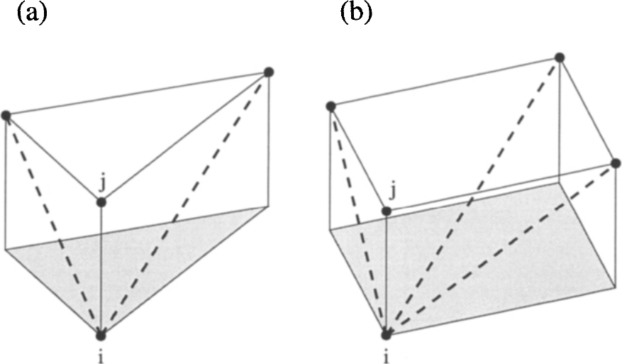
图5.15:用于计算节点\(i\)处梯度的虚拟边(虚线)[49]。图例:所示为边界上(阴影)的棱柱单元(a)与六面体单元(b);\(i\)、\(j\)——节点;虚线为虚拟边。
5.3.5 Limiter Functions 限制器函数[cfd-5-3-5]
二阶及更高阶的上风空间离散需要使用所谓的限制器(limiter)或限制器函数(limiter function)ï¼以防止在大梯度区域(如激波处)产生振荡与虚假解。因此ï¼我们至少要达到单调性保持(monotonicity preserving)的格式。这意味着流场中的极大值必须不增ï¼极小值必须不减ï¼并且在时间推进过程中不得产生新的局部极值。对于结构网格上的上风格式ï¼我们已在4.3.5小节讨论过这一点。en
Second- and higher-order upwind spatial discretisations require the use of so-called limiters or limiter functions in order to prevent the generation of oscillations and spurious solutions in regions with large gradients (e.g., at shocks). Hence, what we want to achieve is at least a monotonicity preserving scheme. This means that maxima in the flow field must be non-increasing, minima non-decreasing, and no new local extrema may be created during the time evolution. We discussed this point in Subsection 4.3.5 for the case of structured upwind discretisation schemes.
在非结构网格上ï¼限制器的目的是减小用于重构控制体面左、右状态的梯度。限制器函数在强间断处必须为零ï¼以得到保证单调性的一阶上风格式。把限制器置零即导致式(5.38)的常数重构。当然ï¼在流场光滑区域必须保留原来的无限制重构ï¼以使数值耗散尽可能低。下面我们将描述两种广泛使用的限制器函数——即Barth与Jespersen的限制器[30]ï¼以及Venkatakrishnan的限制器[68]、[69]。en
On unstructured grids, the purpose of a limiter is to reduce the gradients used to reconstruct the left and right state at the face of the control volume. The limiter function must be zero at strong discontinuities, in order to obtain a first-order upwind scheme which guarantees monotonicity. Setting the limiter to zero leads to the constant reconstruction of Eq. (5.38). Of course, the original unlimited reconstruction has to be retained in smooth flow regions, in order to keep the amount of numerical dissipation as low as possible. In the following, we shall describe two widely used limiter functions - namely the limiters of Barth and Jespersen [30], and of Venkatakrishnan [68], [69].
Limiter of Barth and Jespersen Barth与Jespersen限制器
限制器函数在非结构网格上的首次实现见于文献[30]。对中点对偶格式ï¼它定义在节点\(i\)处为en
The first implementation of a limiter function on unstructured grids was presented in Ref. [30]. In the case of the median-dual scheme, it is defined at the node \(i\) as
其中的缩写为en
with the abbreviations
在式(5.64)与式(5.65)中,\(\min_j\)或\(\max_j\)表示节点\(i\)的所有直接邻居\(j\)(即所有与\(i\)通过边相连的节点)上的最小值或最大值。此外ï¼边向量\(\vec{r}_{ij}\)(示于图5.9或图5.13b)按式(5.43)定义。最后,\(U_j\)表示某个相邻节点\(j\)处的标量。对单元中心格式ï¼与上面类似的公式成立ï¼只需把节点指标换成单元指标ï¼并且en
In Equations (5.64) and (5.65), \(\min_j\) or \(\max_j\) means the minimum or maximum value of all direct neighbours \(j\) of node \(i\) (i.e., all nodes connected to \(i\) by an edge). Furthermore, the edge vector \(\vec{r}_{ij}\), which is shown in Fig. 5.9 or in Fig. 5.13b, is defined according to Eq. (5.43). Finally, \(U_j\) denotes a scalar quantity at some neighbouring node \(j\). Similar formulae to those above hold for the cell-centred scheme with cell instead of node indices and with
其中\(\vec{r}_L\)表示从单元形心指向相应单元面中点的向量。为了避免式(5.64)中除以非常小的\(\Delta_2\)值ï¼最好把\(\Delta_2\)改写为\(\mathrm{Sign}(\Delta_2)(\left|\Delta_2\right| + \omega)\)ï¼其中\(\omega\)约为机器精度[68]。en
where \(\vec{r}_L\) denotes the vector from the cell-centroid to the midpoint of the corresponding cell face. In order to avoid division by a very small value of \(\Delta_2\) in Eq. (5.64), it is better to modify \(\Delta_2\) as \(\mathrm{Sign}(\Delta_2)(\left|\Delta_2\right| + \omega)\), where \(\omega\) is approximately the machine accuracy [68].
Barth限制器强制解单调。但它耗散较大ï¼倾向于抹平间断。另一个问题是:在流场光滑区域ï¼数值噪声也会激活限制器。这通常阻碍向定常状态的完全收敛[68]、[38]。因此,Venkatakrishnan的限制器函数变得更为流行。en
Barth's limiter enforces a monotone solution. However, it is rather dissipative and it tends to smear discontinuities. A further problem presents the activation of the limiter due to numerical noise in smooth flow regions. This usually prevents the full convergence to steady state [68], [38]. Therefore, the limiter function due to Venkatakrishnan became more popular.
Venkatakrishnan's limiter Venkatakrishnan限制器
Venkatakrishnan限制器[68]、[69]因其优越的收敛特性而被广泛使用。该限制器按下列因子缩减顶点\(i\)处重构的梯度\(\nabla U\)en
Venkatakrishnan's limiter [68], [69] is widely used because of its superior convergence properties. The limiter reduces the reconstructed gradient \(\nabla U\) at the vertex \(i\) by the factor
其中en
where
在上面的式(5.68)中,\(U_{max}\)与\(U_{min}\)表示所有周围节点\(j\)(包括节点\(i\)本身)的最大值/最小值。\(U_{max}\)、\(U_{min}\)与\(\Delta_2\)的定义见式(5.65)。参数\(\epsilon^{2}\)用于控制限制的强度。把\(\epsilon^{2}\)置零会导致完全限制ï¼但这可能使收敛停滞。相反ï¼若把\(\epsilon^{2}\)取得很大ï¼限制器函数将返回约等于1的值ï¼于是完全没有限制ï¼解中可能出现波动。实践中发现,\(\epsilon^{2}\)应与局部长度尺度成比例ï¼即en
In the above Eq. (5.68), \(U_{max}\) and \(U_{min}\) stand for the minimum/maximum values of all surrounding nodes \(j\) and including the node \(i\) itself. Definitions of \(U_{max}\), \(U_{min}\) and \(\Delta_2\) are given in Eq. (5.65). The parameter \(\epsilon^{2}\) is intended to control the amount of limiting. Setting \(\epsilon^{2}\) to zero results in full limiting, but this may stall the convergence. Contrary to that, if \(\epsilon^{2}\) is set to a large value, the limiter function will return a value of about unity. Hence, there will be no limiting at all and wiggles could occur in the solution. In practice, it was found that \(\epsilon^{2}\) should be proportional to a local length scale, i.e.,
其中\(K\)为\(\mathcal{O}(1)\)量级的常数,\(\Delta h\)例如取控制体体积的立方根(二维取面积的平方根)。需要注意ï¼限制器函数(5.67)必须用无量纲量定义。式(5.69)中系数\(K\)对激波分辨率的影响示于图5.16。可以看到ï¼完全限制\((K = 0)\)的解与\(K = 5\)的解相同。然而ï¼显式时间推进格式在\(K = 0\)时只收敛了约三个数量级ï¼而\(K = 5\)时收敛到机器零(图5.17)。图5.16还表明ï¼随着\(K\)增大ï¼解逐渐变为无限制ï¼表现为激波处的过冲不断增大。en
where \(K\) is a constant of \(\mathcal{O}(1)\) and \(\Delta h\) is for example the cube-root of the volume (square-root of the area in 2D) of the control volume. It is important to notice that the limiter function (5.67) must be defined with non-dimensional quantities. The influence of the coefficient \(K\) in Eq. (5.69) on the resolution of a shock is demonstrated in Fig. 5.16. It can be seen that the fully limited \((K = 0)\) and the solution for \(K = 5\) are identical. However, the explicit time-stepping scheme converged only about three orders of magnitude for \(K = 0\), whereas for \(K = 5\) it converged to machine zero (Fig. 5.17). Figure 5.16 also shows that the solution becomes gradually unlimited with increasing values of \(K\). This manifests itself as an increasing overshoot at the shock.
计算上述任一限制器函数的工作量都相当大。为了算出\(U_{max}\)、\(U_{min}\)以及限制器\(\Psi\)本身ï¼需要对边循环两次(单元中心格式则对面循环)ï¼并对节点(单元)循环一次。此外,\(U_{max}\)、\(U_{min}\)与\(\Psi\)必须按节点(单元)逐一存储ï¼而且要为每个流动变量分别存储。en
The computational effort for the evaluation of one of the above limiter functions is relatively high. Two loops over edges (faces in the case of the cell-centred scheme) and one loop over nodes (cells) are necessary in order to compute \(U_{max}\), \(U_{min}\) as well as the limiter \(\Psi\) itself. Furthermore, \(U_{max}\), \(U_{min}\) and \(\Psi\) have to be stored node-(cell-)wise, separately for each flow variable.
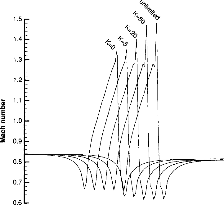
图5.16:Venkatakrishnan限制器中常数\(K\)(由式(5.67)给出)对圆弧无黏绕流解的影响。图例:纵轴为马赫数(Mach number);曲线自左至右对应\(K = 0\)、\(K = 5\)、\(K = 20\)、\(K = 50\)及无限制(unlimited)。
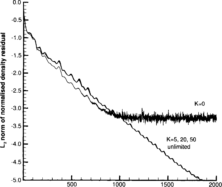
图5.17:Venkatakrishnan限制器中常数\(K\)对圆弧无黏绕流收敛历史的影响。图例:纵轴为归一化密度残差的\(L_2\)范数ï¼横轴为迭代次数(Iterations);\(K = 0\)时残差停滞;\(K = 5\)、\(20\)、\(50\)与无限制(unlimited)则收敛到机器零。
5.4 Discretisation of the Viscous Fluxes 黏性通量的离散[cfd-5-4]
为了计算式(5.2)中的扩散通量\(\vec{F}_v\)ï¼必须知道控制体面上的流动量及其一阶导数。为了得到一致的空间离散并简化数据结构ï¼黏性通量的控制体宜选取成与对流通量的相同。由于黏性通量的椭圆性质ï¼速度分量\((u, v, w)\)、动力黏度\(\mu\)以及热传导系数\(k\)的值——即计算黏性项(2.23)、(2.24)与应力(2.15)所需要的量——直接在面上取平均。于是ï¼对单元中心格式(图5.13a)ï¼控制体面\(IJ\)上的值由下式给出en
In order to evaluate the diffusive fluxes \(\vec{F}_v\) in Eq. (5.2), flow quantities and their first derivatives have to be known at the faces of the control volumes. The control volume for the viscous fluxes is conveniently chosen to be the same as for the convective fluxes in order to obtain a consistent spatial discretisation and to simplify the data structure. Because of the elliptic nature of the viscous fluxes, values of the velocity components \((u, v, w)\), the dynamic viscosity \(\mu\), and of the heat conduction coefficient \(k\), which are required for the computation of the viscous terms (2.23), (2.24) and of the stresses (2.15), are simply averaged at a face. Thus, in the case of the cell-centred scheme (Fig. 5.13a), the values at the face \(IJ\) of the control volume result from
其中\(U\)为上述任一流动变量。中点对偶格式在面\(ij\)处也有类似表达式——见图5.13b。en
where \(U\) is any of the above flow variables. A similar expression holds in the case of the median-dual scheme for the face \(ij\) - see Fig. 5.13b.
剩下的任务是计算式(2.15)中速度分量的一阶导数(梯度)以及式(2.24)中温度的梯度。这可以用以下两种方法之一完成:
- 基于单元的梯度;或
- 梯度平均。
en
The remaining task is the evaluation of the first derivatives (gradients) of the velocity components in Eq. (2.15) and of temperature in Eq. (2.24). This can be accomplished in one of two ways, i.e., by using
- element-based gradients, or
- average of gradients.
下面我们将进一步了解这两种方法。en
In the following, we shall learn more about both approaches.
5.4.1 Element-Based Gradients 基于单元的梯度[cfd-5-4-1]
这类梯度计算的共同特点是:必须存储关于网格单元的信息ï¼或存储与单元几何有关的一些系数。因此ï¼我们必须把数据结构扩展到前面为对流通量介绍的基于面/边的表述之外。下面讨论用于单元中心离散与中点对偶离散的三种成熟方法。en
A common feature of this type of gradient computation is the necessity to store either information about the grid elements or some coefficients related to the geometry of the elements. Hence, we have to extend the data structure beyond the face-/edge-based formulation presented earlier for the convective fluxes. Below, we discuss three well-established methods for the cell-centred and the median-dual discretisation.
Face-Centred Control Volume 面心控制体
计算控制体面上梯度的一种可能办法ï¼是定义一个以该面为中心的辅助控制体ï¼并使用Green-Gauss定理。我们已在4.4节的结构网格有限体积离散框架内讨论过这一方法。例如ï¼对中点对偶格式ï¼可以把边中点处的梯度计算为共享该边的所有单元梯度的体积平均[70]。基于单元的梯度按式(5.49)计算:遍历所有网格单元ï¼并把梯度累加到各条边上。单元面上的\(U\)值通过平均节点值得到ï¼方式与式(5.53)类似。这种方法在内存与运算次数方面代价相对较高ï¼但可用于任意单元组合。en
One possible way of evaluating the gradients at a face of the control volume is to define an auxiliary control volume centred at the face and to employ the Green-Gauss theorem. We already discussed this approach in Section 4.4 in the framework of the structured finite volume discretisation. For example, in the case of the median-dual scheme we can compute the gradient at the edge-midpoint as the volume average of gradients for all elements which share the edge [70]. The element-based gradients are evaluated according to Eq. (5.49) by looping over all grid cells and accumulating the gradients at the edges. The values of \(U\) at the cell-faces are obtained by averaging the nodal values, in a manner similar to Eq. (5.53). This approach is relatively costly in terms of the memory and the number of operations. However, it can be implemented for any mix of grid elements.
Approximate Galerkin Finite Element Approach 近似Galerkin有限元方法
另一种适用于中点对偶格式的方法由Galerkin有限元方法导出[31]。大体上说ï¼该方法把梯度在控制体表面上的积分转化为在中心节点处计算Hessian矩阵(二阶导数)。此时黏性项遵循笛卡尔坐标系下Navier-Stokes方程的微分形式(式(A.4)ï¼其中\(\xi = x\)、\(\eta = y\)、\(\zeta = z\)且\(J^{-1} = 1\))ï¼其中包含如下形式的项en
Another methodology, which is applicable to the median-dual scheme, was derived from the Galerkin finite element method [31]. Basically speaking, the approach transforms the integration of gradients over the surface of the control volume into an evaluation of the Hessian matrix (second derivatives) at the central node. The viscous terms then follow the differential form of the Navier-Stokes equations in Cartesian coordinates (Eq. (A.4) with \(\xi = x\), \(\eta = y\), \(\zeta = z\) and \(J^{-1} = 1\)), which contains terms such as
其中\(\partial_m(\cdot) = \partial(\cdot)/\partial m\)。这样ï¼黏性通量就无需再沿控制体的面进行积分。en
with \(\partial_m(\cdot) = \partial(\cdot)/\partial m\). Hence, no further integration of the viscous fluxes over the faces of the control volume is required.
原始格式是针对纯三角形/四面体网格建立的。它采用包含相应节点的所有单元的并集。为了简化实现ï¼动力黏度系数由节点值平均得到ï¼这是与Galerkin方法的一个不同之处。于是ï¼二阶导数可在节点\(i\)处按如下方式计算[71]en
The original scheme was formulated for purely triangular/tetrahedral grids. It employs a union of all elements that contain the particular node. In order to simplify the implementation, the dynamic viscosity coefficient is averaged from the nodal values, which is a difference to the Galerkin method. Then, the second derivatives can be evaluated at node \(i\) as follows [71]
体积\(\Omega'\)包含共享节点\(i\)的所有四面体。式(5.71)中的系数矩阵\(\alpha\)关于对角线对称[71]ï¼即\(\alpha_{xy} = \alpha_{yx}\)、\(\alpha_{xz} = \alpha_{zx}\)、\(\alpha_{yz} = \alpha_{zy}\)。因此ï¼每条边只需存储六个系数。系数由下式给出[71]en
The volume \(\Omega'\) contains all tetrahedra which share the node \(i\). The coefficient matrix \(\alpha\) in Eq. (5.71) is symmetric about the diagonal [71], i.e., \(\alpha_{xy} = \alpha_{yx}\), \(\alpha_{xz} = \alpha_{zx}\), and \(\alpha_{yz} = \alpha_{zy}\), respectively. Thus, it is necessary to store only six coefficients for each edge. The coefficients are given by [71]
其中\(n\)、\(k\)表示\(x\)、\(y\)、\(z\)下标,\((\vec{S}_e^{i})_k\)与\((\vec{S}_e^{j})_n\)表示图5.18所示外侧面向量\(\vec{S}_e^{i}\)、\(\vec{S}_e^{j}\)的分量。求和遍及共享边\(ij\)的所有四面体(各自体积为\(\Omega_e\))。若网格静止ï¼系数可在预处理阶段计算。一个可取之处是:可以使用与对流通量相同的基于边的数据结构。en
where \(n\), \(k\) denote the \(x\), \(y\), \(z\) subscripts, and \((\vec{S}_e^{i})_k\), \((\vec{S}_e^{j})_n\) represent components of the outer face vectors \(\vec{S}_e^{i}\), \(\vec{S}_e^{j}\) displayed in Fig. 5.18. The summation is carried out over all tetrahedra (with particular volumes \(\Omega_e\)) which share the edge \(ij\). If the grid is stationary, the coefficients can be computed in a pre-processing step. A desirable feature is that the same edge-based data structure can be employed as for the convective fluxes.
不过这种方法的缺点在于:完全的黏性项只在三角形或四面体网格上得以保留。对棱柱或六面体之类的单元ï¼该技术简化为三个坐标方向上的TSL型Navier-Stokes方程近似[8]。文献[72]提出了一种保留完全黏性项的非单纯形单元推广。但此时便无法再使用高效的基于边的数据结构ï¼因为扩展的模板涉及与点\(i\)没有边相连的节点。en
The disadvantage of this approach is however that the full viscous terms are retained only on triangular or tetrahedral grids. For elements like prisms or hexahedra, this technique simplifies to a TSL-like approximation of the Navier-Stokes equations in all three coordinate directions [8]. An extension to non-simplex elements which conserves the full viscous terms was presented in [72]. But the efficient edge-based data structure can then no longer be used since the extended stencil involves nodes not connected by an edge to point \(i\).
Average of Nodal Values 节点值平均
该方案面向单元中心型控制体与纯四面体网格。它采用文献[61]所引入模板的一个修改版本[4]来计算单元面上的梯度。该方法基于定义单元面的三个节点上数值的平均ï¼并结合单元形心处的量。单元面上的一阶导数由下列线性方程组的解得到[4]en
This scheme is intended for the cell-centred type of control volume and purely tetrahedral grids. It employs a modified version [4] of the stencil introduced in [61] to evaluate the gradients at the cell faces. The approach is based on an average of the values at the three nodes which define the cell face, combined with the quantities at the cell centroids. The first derivatives at a cell face result from the solution of the linear system of equations [4]
参照图5.19ï¼下标\(I\)、\(J\)表示单元形心ï¼下标\(1\)、\(2\)、\(3\)分别表示节点\(P_1\)、\(P_2\)与\(P_3\)。节点处的流动变量可由逆距离加权(式(5.45))或伪拉普拉斯加权[2](类似于式(5.24))确定。en
Referring to Fig. 5.19, the subscripts \(I\), \(J\) denote the cell-centroids, and the subscripts \(1\), \(2\), \(3\) stand for the nodes \(P_1\), \(P_2\) and \(P_3\), respectively. Flow variables at the nodes can be determined either from the inverse-distance weighting (Eq. (5.45)) or by the pseudo-Laplacian weighting [2] (similar to Eq. (5.24)).
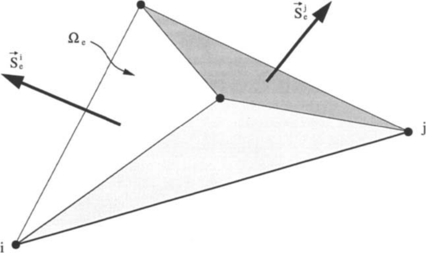
图5.18:节点\(i\)处的黏性项:体积为\(\Omega_e\)的四面体ï¼以及计算与边\(ij\)相关系数所涉及的三角面[71]。图例:\(i\)、\(j\)——节点;\(\Omega_e\)——共享边\(ij\)的四面体的体积;\(\vec{S}_e^{i}\)、\(\vec{S}_e^{j}\)——外侧面向量。
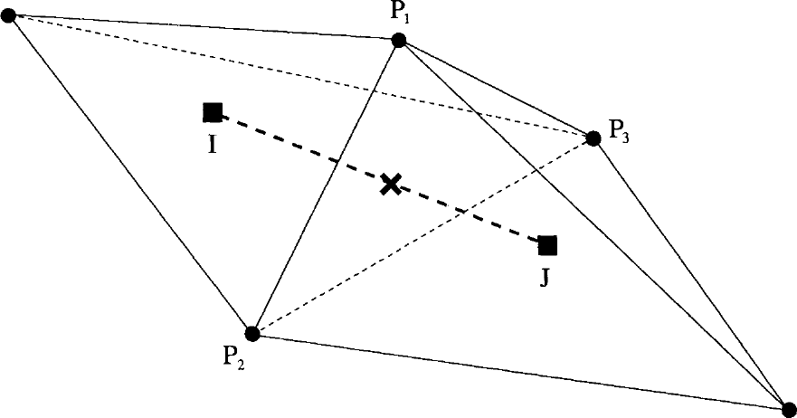
图5.19:单元中心格式:四面体网格上梯度计算的模板[4]。图例:\(I\)、\(J\)——单元形心;\(P_1\)、\(P_2\)、\(P_3\)——定义单元面的节点;叉号表示为计算黏性通量而求梯度的位置(面\(P_1P_2P_3\)的中点);虚线为两形心连线。
5.4.2 Average of Gradients 梯度平均[cfd-5-4-2]
这种方法特别有吸引力ï¼因为它只需要基本的基于面或边的数据结构ï¼不需要额外存储。然而ï¼正如文献[71]等指出的ï¼它导致一个权重分布不利的宽模板[49]。此外,[49]中证明ï¼该模板使解在四边形或六面体网格上可能发生失联(decoupling)。en
This approach is particularly attractive, because it requires only the basic face- or edge-based data structure and no additional storage. However, as it was pointed out, e.g., in Ref. [71], it leads to a wide stencil with an unfavourable distribution of the weights [49]. Furthermore, it was demonstrated in [49] that the stencil allows for the decoupling of the solution on quadrilateral or hexahedral grids.
利用沿单元形心连线方向的方向导数(对单元中心格式)ï¼可以改善该方法的性质ï¼尤其可以防止失联ï¼即en
The properties of the method can be improved, and particularly the decoupling can be prevented, by using the directional derivative along the connection between the cell-centroids (in the case of the cell-centred scheme), i.e.,
其中\(\ell_{IJ}\)表示两个单元形心\(I\)与\(J\)之间的距离(图5.19中的虚线)。对中点对偶格式也有类似表达式ï¼其中\(\vec{r}_{ij}\)按式(5.43)定义。定义沿\(I\)与\(J\)连线的单位向量\(\vec{t}_{IJ}\)为en
where \(\ell_{IJ}\) represents the distance between the both cell-centroids \(I\) and \(J\) (dashed line in Fig. 5.19). A similar expression holds also for the median-dual scheme with \(\vec{r}_{ij}\) according to Eq. (5.43). With the definition of the unit vector \(\vec{t}_{IJ}\) along the line connecting \(I\) and \(J\),
修正的平均可写为[74]、[75]en
the modified average may be written as [74], [75]
其中\(\overline{\nabla U}_{IJ}\)由式(5.74)给出。这一修正在四面体以及棱柱或六面体网格上都导致强耦合的模板[49]。修正后的方法仍与基于面/边的数据结构相容ï¼且不需要额外存储。因此ï¼只要控制体内部的梯度反正要用于对流通量的计算ï¼它就比基于单元的方法更有吸引力。en
where \(\overline{\nabla U}_{IJ}\) is given by Eq. (5.74). The modification leads to strongly coupled stencils on tetrahedral as well as on prismatic or hexahedral grids [49]. The modified approach is also still compatible with the face-/edge-based data structure and requires no additional storage. It is therefore more attractive than the element-based methodology, provided the gradients inside control volumes are utilised for the convective fluxes anyway.