5.4.1 Element-Based Gradients 基于单元的梯度[cfd-5-4-1]
这类梯度计算的共同特点是:必须存储关于网格单元的信息ï¼或存储与单元几何有关的一些系数。因此ï¼我们必须把数据结构扩展到前面为对流通量介绍的基于面/边的表述之外。下面讨论用于单元中心离散与中点对偶离散的三种成熟方法。en
A common feature of this type of gradient computation is the necessity to store either information about the grid elements or some coefficients related to the geometry of the elements. Hence, we have to extend the data structure beyond the face-/edge-based formulation presented earlier for the convective fluxes. Below, we discuss three well-established methods for the cell-centred and the median-dual discretisation.
Face-Centred Control Volume 面心控制体
计算控制体面上梯度的一种可能办法ï¼是定义一个以该面为中心的辅助控制体ï¼并使用Green-Gauss定理。我们已在4.4节的结构网格有限体积离散框架内讨论过这一方法。例如ï¼对中点对偶格式ï¼可以把边中点处的梯度计算为共享该边的所有单元梯度的体积平均[70]。基于单元的梯度按式(5.49)计算:遍历所有网格单元ï¼并把梯度累加到各条边上。单元面上的\(U\)值通过平均节点值得到ï¼方式与式(5.53)类似。这种方法在内存与运算次数方面代价相对较高ï¼但可用于任意单元组合。en
One possible way of evaluating the gradients at a face of the control volume is to define an auxiliary control volume centred at the face and to employ the Green-Gauss theorem. We already discussed this approach in Section 4.4 in the framework of the structured finite volume discretisation. For example, in the case of the median-dual scheme we can compute the gradient at the edge-midpoint as the volume average of gradients for all elements which share the edge [70]. The element-based gradients are evaluated according to Eq. (5.49) by looping over all grid cells and accumulating the gradients at the edges. The values of \(U\) at the cell-faces are obtained by averaging the nodal values, in a manner similar to Eq. (5.53). This approach is relatively costly in terms of the memory and the number of operations. However, it can be implemented for any mix of grid elements.
Approximate Galerkin Finite Element Approach 近似Galerkin有限元方法
另一种适用于中点对偶格式的方法由Galerkin有限元方法导出[31]。大体上说ï¼该方法把梯度在控制体表面上的积分转化为在中心节点处计算Hessian矩阵(二阶导数)。此时黏性项遵循笛卡尔坐标系下Navier-Stokes方程的微分形式(式(A.4)ï¼其中\(\xi = x\)、\(\eta = y\)、\(\zeta = z\)且\(J^{-1} = 1\))ï¼其中包含如下形式的项en
Another methodology, which is applicable to the median-dual scheme, was derived from the Galerkin finite element method [31]. Basically speaking, the approach transforms the integration of gradients over the surface of the control volume into an evaluation of the Hessian matrix (second derivatives) at the central node. The viscous terms then follow the differential form of the Navier-Stokes equations in Cartesian coordinates (Eq. (A.4) with \(\xi = x\), \(\eta = y\), \(\zeta = z\) and \(J^{-1} = 1\)), which contains terms such as
其中\(\partial_m(\cdot) = \partial(\cdot)/\partial m\)。这样ï¼黏性通量就无需再沿控制体的面进行积分。en
with \(\partial_m(\cdot) = \partial(\cdot)/\partial m\). Hence, no further integration of the viscous fluxes over the faces of the control volume is required.
原始格式是针对纯三角形/四面体网格建立的。它采用包含相应节点的所有单元的并集。为了简化实现ï¼动力黏度系数由节点值平均得到ï¼这是与Galerkin方法的一个不同之处。于是ï¼二阶导数可在节点\(i\)处按如下方式计算[71]en
The original scheme was formulated for purely triangular/tetrahedral grids. It employs a union of all elements that contain the particular node. In order to simplify the implementation, the dynamic viscosity coefficient is averaged from the nodal values, which is a difference to the Galerkin method. Then, the second derivatives can be evaluated at node \(i\) as follows [71]
体积\(\Omega'\)包含共享节点\(i\)的所有四面体。式(5.71)中的系数矩阵\(\alpha\)关于对角线对称[71]ï¼即\(\alpha_{xy} = \alpha_{yx}\)、\(\alpha_{xz} = \alpha_{zx}\)、\(\alpha_{yz} = \alpha_{zy}\)。因此ï¼每条边只需存储六个系数。系数由下式给出[71]en
The volume \(\Omega'\) contains all tetrahedra which share the node \(i\). The coefficient matrix \(\alpha\) in Eq. (5.71) is symmetric about the diagonal [71], i.e., \(\alpha_{xy} = \alpha_{yx}\), \(\alpha_{xz} = \alpha_{zx}\), and \(\alpha_{yz} = \alpha_{zy}\), respectively. Thus, it is necessary to store only six coefficients for each edge. The coefficients are given by [71]
其中\(n\)、\(k\)表示\(x\)、\(y\)、\(z\)下标,\((\vec{S}_e^{i})_k\)与\((\vec{S}_e^{j})_n\)表示图5.18所示外侧面向量\(\vec{S}_e^{i}\)、\(\vec{S}_e^{j}\)的分量。求和遍及共享边\(ij\)的所有四面体(各自体积为\(\Omega_e\))。若网格静止ï¼系数可在预处理阶段计算。一个可取之处是:可以使用与对流通量相同的基于边的数据结构。en
where \(n\), \(k\) denote the \(x\), \(y\), \(z\) subscripts, and \((\vec{S}_e^{i})_k\), \((\vec{S}_e^{j})_n\) represent components of the outer face vectors \(\vec{S}_e^{i}\), \(\vec{S}_e^{j}\) displayed in Fig. 5.18. The summation is carried out over all tetrahedra (with particular volumes \(\Omega_e\)) which share the edge \(ij\). If the grid is stationary, the coefficients can be computed in a pre-processing step. A desirable feature is that the same edge-based data structure can be employed as for the convective fluxes.
不过这种方法的缺点在于:完全的黏性项只在三角形或四面体网格上得以保留。对棱柱或六面体之类的单元ï¼该技术简化为三个坐标方向上的TSL型Navier-Stokes方程近似[8]。文献[72]提出了一种保留完全黏性项的非单纯形单元推广。但此时便无法再使用高效的基于边的数据结构ï¼因为扩展的模板涉及与点\(i\)没有边相连的节点。en
The disadvantage of this approach is however that the full viscous terms are retained only on triangular or tetrahedral grids. For elements like prisms or hexahedra, this technique simplifies to a TSL-like approximation of the Navier-Stokes equations in all three coordinate directions [8]. An extension to non-simplex elements which conserves the full viscous terms was presented in [72]. But the efficient edge-based data structure can then no longer be used since the extended stencil involves nodes not connected by an edge to point \(i\).
Average of Nodal Values 节点值平均
该方案面向单元中心型控制体与纯四面体网格。它采用文献[61]所引入模板的一个修改版本[4]来计算单元面上的梯度。该方法基于定义单元面的三个节点上数值的平均ï¼并结合单元形心处的量。单元面上的一阶导数由下列线性方程组的解得到[4]en
This scheme is intended for the cell-centred type of control volume and purely tetrahedral grids. It employs a modified version [4] of the stencil introduced in [61] to evaluate the gradients at the cell faces. The approach is based on an average of the values at the three nodes which define the cell face, combined with the quantities at the cell centroids. The first derivatives at a cell face result from the solution of the linear system of equations [4]
参照图5.19ï¼下标\(I\)、\(J\)表示单元形心ï¼下标\(1\)、\(2\)、\(3\)分别表示节点\(P_1\)、\(P_2\)与\(P_3\)。节点处的流动变量可由逆距离加权(式(5.45))或伪拉普拉斯加权[2](类似于式(5.24))确定。en
Referring to Fig. 5.19, the subscripts \(I\), \(J\) denote the cell-centroids, and the subscripts \(1\), \(2\), \(3\) stand for the nodes \(P_1\), \(P_2\) and \(P_3\), respectively. Flow variables at the nodes can be determined either from the inverse-distance weighting (Eq. (5.45)) or by the pseudo-Laplacian weighting [2] (similar to Eq. (5.24)).
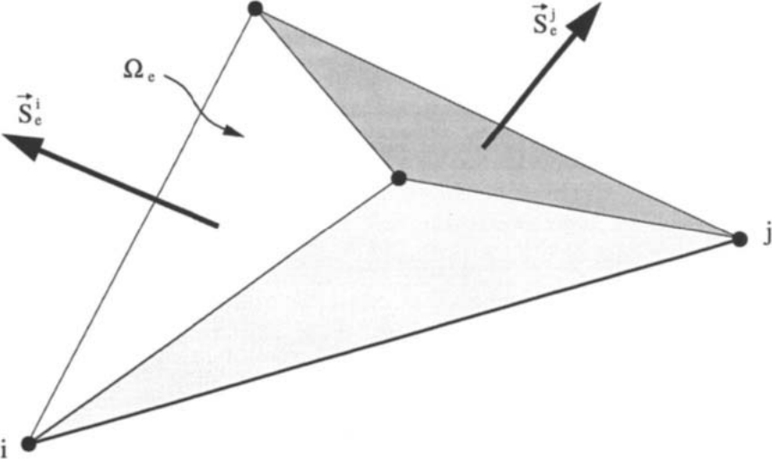
图5.18:节点\(i\)处的黏性项:体积为\(\Omega_e\)的四面体ï¼以及计算与边\(ij\)相关系数所涉及的三角面[71]。图例:\(i\)、\(j\)——节点;\(\Omega_e\)——共享边\(ij\)的四面体的体积;\(\vec{S}_e^{i}\)、\(\vec{S}_e^{j}\)——外侧面向量。
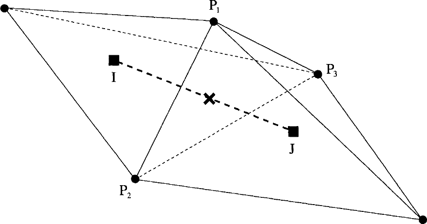
图5.19:单元中心格式:四面体网格上梯度计算的模板[4]。图例:\(I\)、\(J\)——单元形心;\(P_1\)、\(P_2\)、\(P_3\)——定义单元面的节点;叉号表示为计算黏性通量而求梯度的位置(面\(P_1P_2P_3\)的中点);虚线为两形心连线。