5.3.5 Limiter Functions 限制器函数[cfd-5-3-5]
二阶及更高阶的上风空间离散需要使用所谓的限制器(limiter)或限制器函数(limiter function)ï¼以防止在大梯度区域(如激波处)产生振荡与虚假解。因此ï¼我们至少要达到单调性保持(monotonicity preserving)的格式。这意味着流场中的极大值必须不增ï¼极小值必须不减ï¼并且在时间推进过程中不得产生新的局部极值。对于结构网格上的上风格式ï¼我们已在4.3.5小节讨论过这一点。en
Second- and higher-order upwind spatial discretisations require the use of so-called limiters or limiter functions in order to prevent the generation of oscillations and spurious solutions in regions with large gradients (e.g., at shocks). Hence, what we want to achieve is at least a monotonicity preserving scheme. This means that maxima in the flow field must be non-increasing, minima non-decreasing, and no new local extrema may be created during the time evolution. We discussed this point in Subsection 4.3.5 for the case of structured upwind discretisation schemes.
在非结构网格上ï¼限制器的目的是减小用于重构控制体面左、右状态的梯度。限制器函数在强间断处必须为零ï¼以得到保证单调性的一阶上风格式。把限制器置零即导致式(5.38)的常数重构。当然ï¼在流场光滑区域必须保留原来的无限制重构ï¼以使数值耗散尽可能低。下面我们将描述两种广泛使用的限制器函数——即Barth与Jespersen的限制器[30]ï¼以及Venkatakrishnan的限制器[68]、[69]。en
On unstructured grids, the purpose of a limiter is to reduce the gradients used to reconstruct the left and right state at the face of the control volume. The limiter function must be zero at strong discontinuities, in order to obtain a first-order upwind scheme which guarantees monotonicity. Setting the limiter to zero leads to the constant reconstruction of Eq. (5.38). Of course, the original unlimited reconstruction has to be retained in smooth flow regions, in order to keep the amount of numerical dissipation as low as possible. In the following, we shall describe two widely used limiter functions - namely the limiters of Barth and Jespersen [30], and of Venkatakrishnan [68], [69].
Limiter of Barth and Jespersen Barth与Jespersen限制器
限制器函数在非结构网格上的首次实现见于文献[30]。对中点对偶格式ï¼它定义在节点\(i\)处为en
The first implementation of a limiter function on unstructured grids was presented in Ref. [30]. In the case of the median-dual scheme, it is defined at the node \(i\) as
其中的缩写为en
with the abbreviations
在式(5.64)与式(5.65)中,\(\min_j\)或\(\max_j\)表示节点\(i\)的所有直接邻居\(j\)(即所有与\(i\)通过边相连的节点)上的最小值或最大值。此外ï¼边向量\(\vec{r}_{ij}\)(示于图5.9或图5.13b)按式(5.43)定义。最后,\(U_j\)表示某个相邻节点\(j\)处的标量。对单元中心格式ï¼与上面类似的公式成立ï¼只需把节点指标换成单元指标ï¼并且en
In Equations (5.64) and (5.65), \(\min_j\) or \(\max_j\) means the minimum or maximum value of all direct neighbours \(j\) of node \(i\) (i.e., all nodes connected to \(i\) by an edge). Furthermore, the edge vector \(\vec{r}_{ij}\), which is shown in Fig. 5.9 or in Fig. 5.13b, is defined according to Eq. (5.43). Finally, \(U_j\) denotes a scalar quantity at some neighbouring node \(j\). Similar formulae to those above hold for the cell-centred scheme with cell instead of node indices and with
其中\(\vec{r}_L\)表示从单元形心指向相应单元面中点的向量。为了避免式(5.64)中除以非常小的\(\Delta_2\)值ï¼最好把\(\Delta_2\)改写为\(\mathrm{Sign}(\Delta_2)(\left|\Delta_2\right| + \omega)\)ï¼其中\(\omega\)约为机器精度[68]。en
where \(\vec{r}_L\) denotes the vector from the cell-centroid to the midpoint of the corresponding cell face. In order to avoid division by a very small value of \(\Delta_2\) in Eq. (5.64), it is better to modify \(\Delta_2\) as \(\mathrm{Sign}(\Delta_2)(\left|\Delta_2\right| + \omega)\), where \(\omega\) is approximately the machine accuracy [68].
Barth限制器强制解单调。但它耗散较大ï¼倾向于抹平间断。另一个问题是:在流场光滑区域ï¼数值噪声也会激活限制器。这通常阻碍向定常状态的完全收敛[68]、[38]。因此,Venkatakrishnan的限制器函数变得更为流行。en
Barth's limiter enforces a monotone solution. However, it is rather dissipative and it tends to smear discontinuities. A further problem presents the activation of the limiter due to numerical noise in smooth flow regions. This usually prevents the full convergence to steady state [68], [38]. Therefore, the limiter function due to Venkatakrishnan became more popular.
Venkatakrishnan's limiter Venkatakrishnan限制器
Venkatakrishnan限制器[68]、[69]因其优越的收敛特性而被广泛使用。该限制器按下列因子缩减顶点\(i\)处重构的梯度\(\nabla U\)en
Venkatakrishnan's limiter [68], [69] is widely used because of its superior convergence properties. The limiter reduces the reconstructed gradient \(\nabla U\) at the vertex \(i\) by the factor
其中en
where
在上面的式(5.68)中,\(U_{max}\)与\(U_{min}\)表示所有周围节点\(j\)(包括节点\(i\)本身)的最大值/最小值。\(U_{max}\)、\(U_{min}\)与\(\Delta_2\)的定义见式(5.65)。参数\(\epsilon^{2}\)用于控制限制的强度。把\(\epsilon^{2}\)置零会导致完全限制ï¼但这可能使收敛停滞。相反ï¼若把\(\epsilon^{2}\)取得很大ï¼限制器函数将返回约等于1的值ï¼于是完全没有限制ï¼解中可能出现波动。实践中发现,\(\epsilon^{2}\)应与局部长度尺度成比例ï¼即en
In the above Eq. (5.68), \(U_{max}\) and \(U_{min}\) stand for the minimum/maximum values of all surrounding nodes \(j\) and including the node \(i\) itself. Definitions of \(U_{max}\), \(U_{min}\) and \(\Delta_2\) are given in Eq. (5.65). The parameter \(\epsilon^{2}\) is intended to control the amount of limiting. Setting \(\epsilon^{2}\) to zero results in full limiting, but this may stall the convergence. Contrary to that, if \(\epsilon^{2}\) is set to a large value, the limiter function will return a value of about unity. Hence, there will be no limiting at all and wiggles could occur in the solution. In practice, it was found that \(\epsilon^{2}\) should be proportional to a local length scale, i.e.,
其中\(K\)为\(\mathcal{O}(1)\)量级的常数,\(\Delta h\)例如取控制体体积的立方根(二维取面积的平方根)。需要注意ï¼限制器函数(5.67)必须用无量纲量定义。式(5.69)中系数\(K\)对激波分辨率的影响示于图5.16。可以看到ï¼完全限制\((K = 0)\)的解与\(K = 5\)的解相同。然而ï¼显式时间推进格式在\(K = 0\)时只收敛了约三个数量级ï¼而\(K = 5\)时收敛到机器零(图5.17)。图5.16还表明ï¼随着\(K\)增大ï¼解逐渐变为无限制ï¼表现为激波处的过冲不断增大。en
where \(K\) is a constant of \(\mathcal{O}(1)\) and \(\Delta h\) is for example the cube-root of the volume (square-root of the area in 2D) of the control volume. It is important to notice that the limiter function (5.67) must be defined with non-dimensional quantities. The influence of the coefficient \(K\) in Eq. (5.69) on the resolution of a shock is demonstrated in Fig. 5.16. It can be seen that the fully limited \((K = 0)\) and the solution for \(K = 5\) are identical. However, the explicit time-stepping scheme converged only about three orders of magnitude for \(K = 0\), whereas for \(K = 5\) it converged to machine zero (Fig. 5.17). Figure 5.16 also shows that the solution becomes gradually unlimited with increasing values of \(K\). This manifests itself as an increasing overshoot at the shock.
计算上述任一限制器函数的工作量都相当大。为了算出\(U_{max}\)、\(U_{min}\)以及限制器\(\Psi\)本身ï¼需要对边循环两次(单元中心格式则对面循环)ï¼并对节点(单元)循环一次。此外,\(U_{max}\)、\(U_{min}\)与\(\Psi\)必须按节点(单元)逐一存储ï¼而且要为每个流动变量分别存储。en
The computational effort for the evaluation of one of the above limiter functions is relatively high. Two loops over edges (faces in the case of the cell-centred scheme) and one loop over nodes (cells) are necessary in order to compute \(U_{max}\), \(U_{min}\) as well as the limiter \(\Psi\) itself. Furthermore, \(U_{max}\), \(U_{min}\) and \(\Psi\) have to be stored node-(cell-)wise, separately for each flow variable.
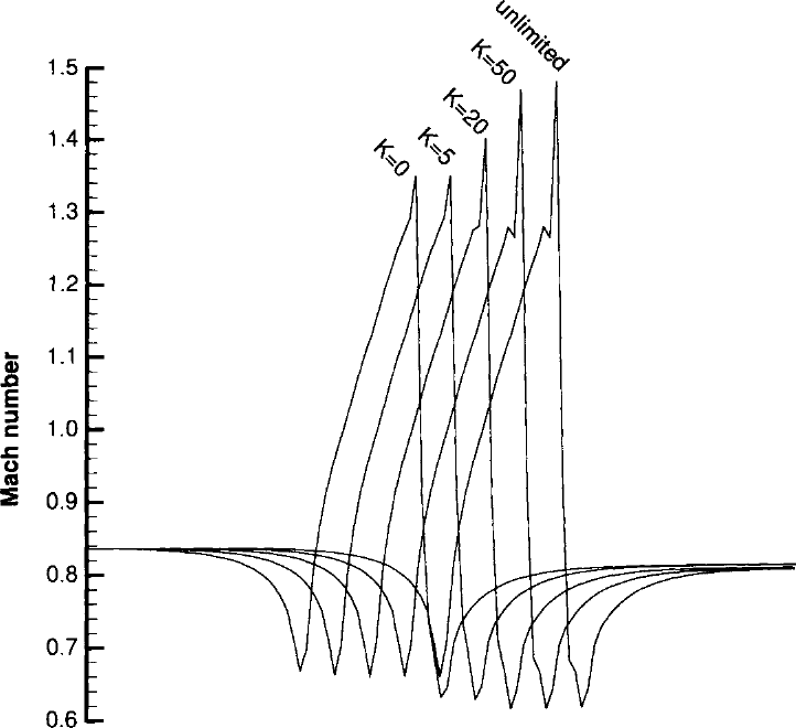
图5.16:Venkatakrishnan限制器中常数\(K\)(由式(5.67)给出)对圆弧无黏绕流解的影响。图例:纵轴为马赫数(Mach number);曲线自左至右对应\(K = 0\)、\(K = 5\)、\(K = 20\)、\(K = 50\)及无限制(unlimited)。
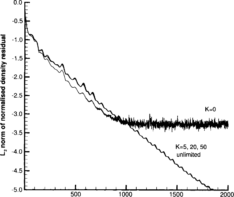
图5.17:Venkatakrishnan限制器中常数\(K\)对圆弧无黏绕流收敛历史的影响。图例:纵轴为归一化密度残差的\(L_2\)范数ï¼横轴为迭代次数(Iterations);\(K = 0\)时残差停滞;\(K = 5\)、\(20\)、\(50\)与无限制(unlimited)则收敛到机器零。