5.3.4 Evaluation of the Gradients 梯度的计算[cfd-5-3-4]
分段线性重构与二次重构的讨论中还遗留一个问题ï¼即梯度的确定。计算黏性通量(5.4节)也需要速度分量与温度的梯度。下面介绍两种方法:第一种基于Green-Gauss定理ï¼第二种利用最小二乘法。en
An open point, which remains from the discussion of the piecewise linear and the quadratic reconstruction, is the determination of the gradient. Gradients of the velocity components and the temperature are also required for the evaluation of the viscous fluxes (Section 5.4). Two approaches will be presented in the following: the first is based on the Green-Gauss theorem, and the second utilises the least-squares method.
Green-Gauss Approach Green-Gauss方法
该方法把某标量函数\(U\)的梯度近似为\(U\)与外指单位法向量的乘积在某个控制体\(\Omega'\)上的面积分ï¼即en
This method approximates the gradient of some scalar function \(U\) as the surface integral of the product of \(U\) with an outward-pointing unit normal vector over some control volume \(\Omega'\), i.e.,
Median-Dual Scheme 中点对偶格式
Barth与Jespersen[30]从Galerkin有限元方法导出了Green-Gauss方法的一种特殊离散。后来,Barth[64]把该离散推广到三维。Barth与Jespersen把式(5.49)应用于在某个节点处相会的所有单元的并集所构成的区域。他们证明ï¼这一方法可以表述成与基于边的数据结构相容的形式。不过ï¼这只对三角形/四面体网格上的中点对偶格式有效。所得公式为en
Barth and Jespersen [30] derived a particular discretisation of the Green-Gauss approach from the Galerkin finite element method. Later on, the discretisation was extended to 3D by Barth [64]. Barth and Jespersen applied Eq. (5.49) to the region formed by the union of the elements meeting at a node. They proved that the approach can be formulated such that it becomes compatible with the edge-based data structure. However, this works only for the median-dual scheme on triangular/tetrahedral grids. The resulting formula reads
这里ï¼式(5.49)中的\(\Omega'\)等于中点对偶控制体\(\Omega\)的体积。求和遍及与节点\(i\)相连的所有\(N_F\)条边。此外,\(\vec{n}_{ij}\)表示按式(5.23)定义的平均单位法向量,\(\Delta S_{ij}\)为总面面积。同一公式(5.50)在二维或三维都适用。需要指出的是ï¼为了得到一致的近似ï¼边界处的求和必须作改变[65](另见8.10节)。en
Here, \(\Omega'\) in Eq. (5.49) equals to the volume of the median-dual control volume \(\Omega\). The summation extends over all \(N_F\) edges incident to node \(i\). Furthermore, \(\vec{n}_{ij}\) denotes the average unit normal vector according to Eq. (5.23), and \(\Delta S_{ij}\) is the total face area, respectively. The same formula (5.50) is applicable in two or in three dimensions. It is important to mention that the summation has to be changed at boundaries in order to obtain a consistent approximation [65] (see also Section 8.10).
Cell-Centred Scheme 单元中心格式
Green-Gauss方法同样可用于单元中心格式。于是ï¼某单元形心\(I\)处的梯度可由下式得到en
We can use the Green-Gauss method in the cell-centred scheme as well. Hence, the gradient at some cell-centroid \(I\) can be obtained from
Mixed Grids 混合网格
用式(5.50)或式(5.51)计算Green-Gauss梯度的主要吸引力在于它与通量计算(如式(5.19))的相似性:这意味着梯度重构不需要额外的数据结构。主要缺点是式(5.50)或式(5.51)的近似在混合网格上会失效。[49]中证明ï¼梯度可能变得很不准确ï¼尤其是在不同单元类型相接之处。对中点对偶格式ï¼如果把式(5.49)中的体积\(\Omega'\)取为与节点\(i\)相关的所有单元的并集ï¼就可以解决这一问题。参照图5.8所示的情形ï¼二维梯度于是由下式给出en
The main attractiveness of the Green-Gauss gradient evaluation by Eq. (5.50) or (5.51) is its similarity to the computation of the fluxes (e.g., Eq. (5.19)). This means that no additional data structures are needed for the reconstruction of gradients. The main disadvantage is that the approximation in Eq. (5.50) or Eq. (5.51), respectively, fails on mixed grids. It was demonstrated in [49] that the gradient can become highly inaccurate, particularly where different element types meet. We can solve the problem in the case of the median-dual scheme when we keep the volume \(\Omega'\) in Eq. (5.49) identical to the union of all cells incident to node \(i\). Referring to the situation sketched in Fig. 5.8, the gradient results then in 2D from
其中取\(i = 0\)ï¼外表面数\(N_O = 6\)(由点\(P_1\)-\(P_6\)给出)ï¼当\(j = 6\)时\(j+1 = 1\)。此外,\(\vec{n}_j\)与\(\Delta S_j\)表示外单元面的单位法向量与面积。在三维中ï¼可用en
with \(i = 0\), the number of outer faces \(N_O = 6\) (given by the points \(P_1\)-\(P_6\)), and \(j+1 = 1\) for \(j = 6\). Furthermore, \(\vec{n}_j\) and \(\Delta S_j\) stand for the unit normal vector and the area of the outer cell faces. In 3D, we can use
这里假设所有的面都是三角形——或天然如此ï¼或经分解而成。同样的补救办法也可用于单元中心格式。此时控制体\(\Omega'\)的表面由远一与远二相邻单元的形心定义[62]、[63]ï¼如图5.14所示。梯度按式(5.52)或式(5.53)计算ï¼只是把节点指标换成单元指标。en
when we assume all faces are triangles - either naturally or by decomposition. The same remedy can be also employed for the cell-centred scheme. The surface of the control volume \(\Omega'\) is then defined by the centroids of the distant-one and distant-two neighbouring cells [62], [63], as it is rendered in Fig. 5.14. The gradient is computed correspondingly to Eq. (5.52) or (5.53) with cell instead of node indices.
这种基于单元的方法的明显缺点是必须增加一种数据结构ï¼以提供中心节点/形心与\(\Omega'\)外表面之间的联系。这样一来ï¼该方法不再是网格透明的(grid-transparentï¼即不再与单元信息无关)ï¼高效的gather-scatter循环也不再可能。这使得下面介绍的最小二乘技术在混合网格上更有吸引力。en
The clear disadvantage of such a cell-based approach is the necessity of an additional data structure, which provides a link between the central node/centroid and the outer faces of \(\Omega'\). Thus, the approach is no longer grid-transparent (i.e., independent of the cell information) and an efficient gather-scatter loop is no longer possible. This renders the least-squares technique, which is described below, more attractive on mixed grids.
在三角形或四面体网格上使用基于边/面的实现(5.50)或(5.51)ï¼在混合网格上使用基于单元的方法(5.52)或(5.53),Green-Gauss方法至少为一阶精度[63]。它还是一致的(consistent)ï¼即线性函数的梯度可计算到舍入误差精度。一阶精度对线性重构已经足够。二次重构所需的任意网格上的二阶精度ï¼可以通过从梯度的一阶近似中减去截断误差的估计来达到[63]。en
Using the edge-/face-based implementation (5.50) or (5.51) on triangular or tetrahedral grids, and the cell-based methodology (5.52) or (5.53) on mixed grids, the Green-Gauss approach is at least first-order accurate [63]. It is also consistent, i.e., the gradient of a linear function is computed to roundoff error. First-order accuracy is sufficient for the linear reconstruction. Second-order accuracy on arbitrary grids, which is required for the quadratic reconstruction, can be achieved by subtracting an estimate of the truncation error from the first-order approximation of the gradient [63].
Least-Squares Approach 最小二乘方法
用最小二乘方法计算梯度最早由Barth引入[64]、[36]。为了说明该方法ï¼考虑中点对偶格式。此时ï¼最小二乘方法基于对与中心节点\(i\)相连的每条边使用一阶泰勒级数近似。沿边\(ij\)的解的变化可由下式计算en
The evaluation of gradients by the least-squares approach was first introduced by Barth [64], [36]. In order to illustrate the method, let us consider the median-dual scheme. Herewith, the least-squares approach is based upon the use of a first-order Taylor series approximation for each edge which is incident to the central node \(i\). The change of the solution along an edge \(ij\) can be computed from
其中\(\Delta(\cdot)_{ij} = (\cdot)_j - (\cdot)_i\),\(\partial_m(\cdot) = \partial(\cdot)/\partial m\)。此外,\(N_A\)表示与\(i\)通过边相连的相邻节点\(j\)的数目,\(\theta_j\)为某个加权系数。权重可以依赖于几何和/或解(参见例如[40])。不过实践中\(\theta_j\)通常取为1。为方便起见ï¼把上述方程组(5.55)简写为en
with \(\Delta(\cdot)_{ij} = (\cdot)_j - (\cdot)_i\) and \(\partial_m(\cdot) = \partial(\cdot)/\partial m\). Further, \(N_A\) denotes the number of adjacent nodes \(j\) connected to \(i\) by an edge and \(\theta_j\) stands for some weighting coefficient. The weights can depend on the geometry and/or on the solution (see, e.g., [40]). However, in practice \(\theta_j\) is usually set to unity. For convenience, we abbreviate the above system (5.55) as
由式(5.56)解出梯度向量\(\vec{x}\)需要对矩阵\(\bar{A}\)求逆。为了防止病态问题(特别是在拉伸网格上),Anderson与Bonhaus建议用Gram-Schmidt过程把\(\bar{A}\)分解为正交矩阵\(\bar{Q}\)与上三角矩阵\(\bar{R}\)的乘积[66]。他们的方法最近在[49]中被推广到三维。于是ï¼式(5.56)的解立即由下式给出en
Solving Eq. (5.56) for the gradient vector \(\vec{x}\) requires the inversion of the matrix \(\bar{A}\). To prevent problems with ill-conditioning (particularly on stretched grids), Anderson and Bonhaus suggested to decompose \(\bar{A}\) into the product of an orthogonal matrix \(\bar{Q}\) and an upper triangular matrix \(\bar{R}\) using the Gram-Schmidt process [66]. Their approach was recently extended to 3D in [49]. Hence, the solution to Eq. (5.56) immediately follows from
用带双下标的小写字母表示矩阵元素ï¼矩阵\(\bar{A} = [\vec{a}_1,\, \vec{a}_2,\, \vec{a}_3]\)的Gram-Schmidt正交化可写为\(\bar{Q} = [\vec{q}_1,\, \vec{q}_2,\, \vec{q}_3]\)ï¼其中en
Using a lower case letter with double subscripts to denote a matrix element, we may write the Gram-Schmidt orthogonalisation of the matrix \(\bar{A} = [\vec{a}_1,\, \vec{a}_2,\, \vec{a}_3]\) as \(\bar{Q} = [\vec{q}_1,\, \vec{q}_2,\, \vec{q}_3]\), where
上三角矩阵\(\bar{R}\)的元素由下式求得en
The entries in the upper triangular matrix \(\bar{R}\) are obtained from
其中权重向量\(\vec{w}_{ij}\)定义为en
with the vector of weights \(\vec{w}_{ij}\) defined as
其中en
where
对单元中心格式ï¼最小二乘方法的表述在形式上保持不变ï¼只需把节点换成单元形心。例子可参见文献[16]。en
The formulation of the least-squares approach remains formally the same for a cell-centred scheme, only the nodes have to be substituted by cell-centroids. An example may be found in Ref. [16].
最小二乘方法在一般网格上为一阶精度[63]。它也是一致的ï¼即无论单元类型如何ï¼线性函数的梯度都能计算到舍入误差精度。因此该方法特别适合混合网格。其计算成本与Green-Gauss方法相当ï¼因为只需在对面/边的单个循环内做一次向量-标量乘法(式(5.60))。不过ï¼我们必须在每个节点处预先计算并存储上三角矩阵\(\bar{R}\)的六个元素(式(5.59))。文献[67]的详细研究表明ï¼为了在高度拉伸且又弯曲的网格上准确近似非线性函数的梯度ï¼式(5.55)、(5.60)中的加权系数\(\theta_j\)必须取为节点\(i\)与\(j\)之间距离的倒数(类似于式(5.45)中的\(\theta_{ij}\))。然而ï¼这对三角形(四面体)网格上的单元中心格式并无帮助[67]。en
The least-squares method is first-order accurate on general grids [63]. It is also consistent, i.e., the gradient of a linear function is computed to roundoff error, regardless of the type of the elements. Therefore, the method is particularly suited to mixed grids. The computational costs are comparable to those of the Green-Gauss approach, since only a vector-scalar multiplication (Eq. (5.60)) is needed within a single loop over faces/edges. However, we have to pre-compute and store the six entries (Eq. (5.59)) of the upper triangular matrix \(\bar{R}\) at each node. A detailed investigation in Ref. [67] revealed that the weighting coefficient \(\theta_j\) in Eqs. (5.55), (5.60) has to be set equal to the inverse of the distance between the nodes \(i\) and \(j\) (similar to \(\theta_{ij}\) in Eq. (5.45)), in order to obtain an accurate approximation for the gradient of a non-linear function on a highly stretched and additionally curved grid. However, this does not help in the case of the cell-centred scheme on triangular (tetrahedral) grids [67].
经验还表明ï¼当黏性壁面上采用棱柱或六面体单元时ï¼中点对偶格式的最小二乘方法需要注意一些问题。考察图5.15ï¼假设我们要计算节点\(i\)处速度分量的梯度。可以看出ï¼只有来自边\(ij\)的贡献是有用的ï¼因为与\(i\)通过边相连的其他节点上\(u = v = w = 0\)。为了扩大模板的支持范围ï¼可以插入所谓的虚拟边(virtual edges)[49]ï¼如图5.15中的虚线所示。虚拟边能显著改善离散格式的精度与稳健性。应当强调ï¼它们只用于梯度重构ï¼而不用于通量计算。en
Experience also shows that the least-squares approach requires some attention in the case of the median-dual scheme, if prismatic or hexahedral cells are employed on a viscous wall. Consider Fig. 5.15 and assume that we want to compute the gradients of the velocity components at node \(i\). It may become obvious that only the contribution from the edge \(ij\) is useful, since at other nodes connected to \(i\) by an edge \(u = v = w = 0\). To increase the support of the stencil, we can insert the so-called virtual edges [49], as they are rendered by the dashed lines in Fig. 5.15. The virtual edges help to improve the accuracy and the robustness of the discretisation scheme considerably. It should be stressed that they are employed only for the gradient reconstruction but not for the flux computation.
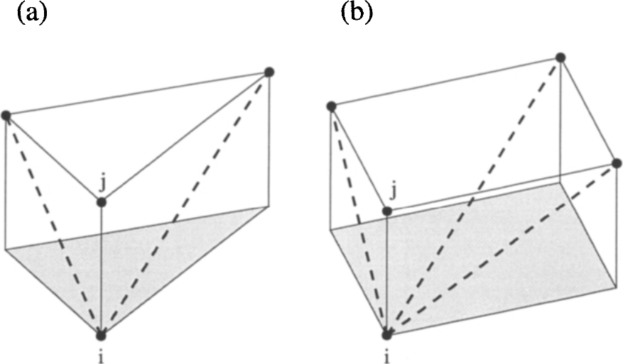
图5.15:用于计算节点\(i\)处梯度的虚拟边(虚线)[49]。图例:所示为边界上(阴影)的棱柱单元(a)与六面体单元(b);\(i\)、\(j\)——节点;虚线为虚拟边。