5.3.3 Solution Reconstruction 解重构[cfd-5-3-3]
正如我们在4.3.2-4.3.4小节中所看到的ï¼上风格式要求在控制体面的左、右两侧给定流动状态。式(5.37)中改进的人工耗散格式也是如此。en
As we saw in Subsections 4.3.2-4.3.4, upwind schemes require flow states to be specified on the left and the right side of a control volume face. The same holds also for the modified artificial dissipation scheme in Eq. (5.37).
作为第一种做法ï¼可以假设解在每个控制体内部为常数。此时左、右状态就是为左、右控制体计算的流动变量。例如ï¼对中点对偶格式(图5.9)ï¼我们会取en
As a first approach, we can assume that the solution is constant inside each control volume. The left and right state are then simply the flow variables computed for the left and the right control volume. For example, in the case of the median-dual scheme (Fig. 5.9) we would set
其中\(U\)代表某个标量流动变量。这样得到的空间离散只有一阶精度。对黏性流动而言ï¼一阶精度的解耗散太大ï¼会导致剪切层过度增长。因此ï¼计算黏性流动必须采用空间精度更高的方法。en
with \(U\) representing some scalar flow variable. This leads to a spatial discretisation which is only first-order accurate. For viscous flows, a first-order accurate solution is too diffusive and leads to an excessive growth of shear layers. Therefore, methods with higher spatial accuracy are a must for the computation of viscous flows.
如果假设解在控制体内部有变化ï¼就可以达到二阶及更高阶精度。二阶精度方法是最常用的高阶方法ï¼它假设解在控制体上按线性方式变化。为了计算左、右状态ï¼需要对所假设的解的变化进行重构。下面我们将讨论线性变化与二次变化重构的最常用方法。关于各种线性重构技术的比较ï¼有兴趣的读者可参阅[38]。en
We can achieve second- and higher-order accuracy if we assume the solution changes over the control volume. For second-order accurate methods, which are the most commonly employed higher-order methods, the solution is assumed to vary in a linear fashion over the control volume. In order to compute the left and right state, a reconstruction of the assumed solution variation becomes necessary. In what follows, we shall discuss the most popular approaches for the reconstruction of linear and quadratic variations. The interested reader is referred to [38] for a comparison of various linear reconstruction techniques.
Reconstruction Based on MUSCL Approach 基于MUSCL方法的重构
达到二阶精度的一种可能途径ï¼是把MUSCL方法[51]推广到非结构网格。当用于中点对偶格式时ï¼该方法为每条边\(ij\)生成两个“虚拟”节点\(i'\)与\(j'\)[52]-[56]。如图5.12所示ï¼这些虚拟节点位于把边\(ij\)向两端各延长一个边长所得线段的端点处。在把解从周围单元(图5.12中着灰色者)插值到虚拟节点之后ï¼便可用MUSCL公式即式(4.46)计算左、右状态。于是,en
One possibility to achieve second-order accuracy consists of the extension of the MUSCL approach [51] to unstructured grids. When applied to the median-dual scheme, the method generates for each edge \(ij\) two "phantom" nodes \(i'\) and \(j'\) [52]-[56]. These phantom nodes are located at the endpoints of the line obtained by extending the edge \(ij\) by its length in both directions as sketched in Fig. 5.12. After the solution is interpolated from the surrounding elements (gray coloured in Fig. 5.12) to the phantom nodes, we can evaluate the left and right state using the MUSCL formulae Eq. (4.46). Hence,
其中前向\((\Delta_{+})\)与后向\((\Delta_{-})\)差分算子定义为en
with forward \((\Delta_{+})\) and the backward \((\Delta_{-})\) difference operators defined as
出现强间断时,MUSCL插值(5.39)必须辅以限制器函数(按照4.3.5小节)。这种方法的一个缺点是必须为每条边存储包含虚拟节点的单元。另一个概念上的缺点是:为一个控制体重构出的梯度并不唯一。此外ï¼在边界处可能出现困难ï¼因为此时某个虚拟点会落在物理域之外。en
The MUSCL interpolation (5.39) has to be enhanced by a limiter function (according to Subsection 4.3.5) in the case of strong discontinuities. A disadvantage of this methodology is the necessity to store for each edge the elements which contain the phantom nodes. A further conceptual disadvantage is that no unique gradient is reconstructed for a control volume. Furthermore, difficulties can arise at boundaries, where one of the phantom points lies outside the physical domain.
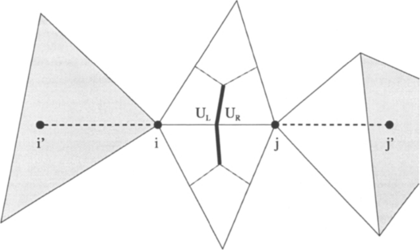
图5.12:基于沿边ij方向的单元插值确定左、右状态(二维中点对偶格式)。图例:\(i'\)、\(i\)、\(j\)、\(j'\)——虚拟节点与边ij的端点;\(U_L\)、\(U_R\)——控制体面上的左状态与右状态;着灰色的单元表示用于插值到虚拟节点的周围单元;虚线表示由边ij向两端延长所得的线段。
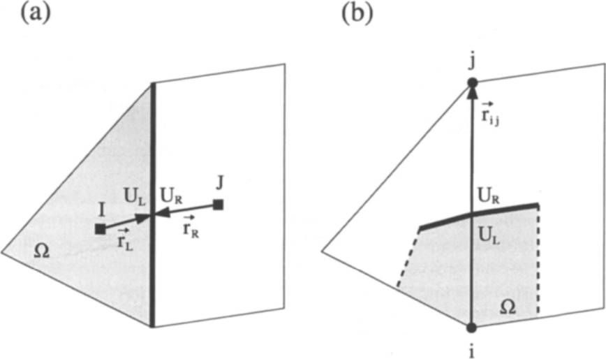
图5.13:二维单元中心格式(a)与中点对偶格式(b)的线性重构。图例:(a)\(I\)、\(J\)——单元形心;\(U_L\)、\(U_R\)——面上的左、右状态;\(\vec{r}_L\)、\(\vec{r}_R\)——由形心指向面中点的向量;\(\Omega\)——控制体。(b)\(i\)、\(j\)——节点;\(\vec{r}_{ij}\)——由节点\(i\)指向\(j\)的边向量;\(U_L\)、\(U_R\)——面上的左、右状态;\(\Omega\)——对偶控制体。
Piecewise Linear Reconstruction 分段线性重构
Barth与Jespersen在[30]中提出了一种与有限元格式密切相关的重构方法。这里假设解在控制体上分段线性分布。于是ï¼对单元中心格式ï¼可由下列关系式求出左、右状态en
Barth and Jespersen presented in [30] a reconstruction method, which is closely related to the finite element schemes. Here, it is assumed that the solution is piecewise linearly distributed over the control volume. Then, we can find the left and right state for a cell-centred scheme from the relations
其中\(\nabla U_I\)是\(U\)(即\([\partial U/\partial x,\, \partial U/\partial y,\, \partial U/\partial z]^T\))在单元中心\(I\)处的梯度,\(\Psi\)表示限制器函数(参见5.3.5小节)。向量\(\vec{r}_L\)与\(\vec{r}_R\)从单元形心指向面中点ï¼如图5.13a所示。en
where \(\nabla U_I\) is the gradient of \(U\) (\(= [\partial U/\partial x,\, \partial U/\partial y,\, \partial U/\partial z]^T\)) at the cell centre \(I\) and \(\Psi\) denotes a limiter function (cf. Subsection 5.3.5), respectively. The vectors \(\vec{r}_L\) and \(\vec{r}_R\) point from the cell-centroid to the face-midpoint, as indicated in Fig. 5.13a.
同样的方法也适用于中点对偶格式[30]ï¼即en
The same approach applies to the median-dual scheme [30], i.e.,
按照图5.9或图5.13b,en
According to Fig. 5.9 or Fig. 5.13b,
表示从节点\(i\)指向节点\(j\)的向量。en
represents the vector from node \(i\) to node \(j\).
容易看出,Barth与Jespersen的方法相当于围绕面相邻的形心/节点作泰勒级数展开并只保留线性项。线性重构在规则网格上形式上为二阶精度[38]。只要梯度\(\nabla U\)的计算没有误差ï¼该格式在任意网格上都能精确重构线性函数。线性重构很可能是各种重构方法中最常用的一种。en
It can be easily seen that the method of Barth and Jespersen corresponds to a Taylor-series expansion around the neighbouring centres/nodes of the face, where only the linear term is retained. The linear reconstruction is formally second-order accurate on regular grids [38]. The scheme reconstructs a linear function exactly on any grid, provided the gradient \(\nabla U\) is evaluated without an error. The linear reconstruction is likely the most popular one among the reconstruction methods.
上述格式需要在单元中心或节点处计算梯度。这既可以用Green-Gauss方法也可以用最小二乘方法实现ï¼二者将在下文5.3.4小节中介绍。此外ï¼限制器函数在非结构网格上的实现将在5.3.5小节中详细描述。en
The above scheme requires the computation of gradients at cell centres or at nodes, respectively. This can be accomplished either by the Green-Gauss or the least-squares approach, which are presented below in Subsection 5.3.4. Furthermore, the implementation of the limiter function on unstructured grids is described in detail in Subsection 5.3.5.
Linear Reconstruction Based on Nodal Weighting Procedure 基于节点加权过程的线性重构
Frink[26]证明ï¼对单元中心格式ï¼在纯三角形或四面体网格上线性重构(5.41)无需显式计算梯度。原因在于这类单元的两个不变几何特征。其一ï¼从任一节点出发穿过单元形心的直线总会与对面(与该节点相对的面)的中点相交。其二ï¼从单元形心到面中点的距离ï¼是从面中点到对面节点距离的四分之一(对三角形为三分之一)。这样ï¼单元中心处的梯度便可用简单有限差分近似[26]。例如ï¼若要重构图5.7a中面中点\(F_3\)处的解ï¼式(5.41)就成为en
It was demonstrated by Frink [26] that for the cell-centred scheme the linear reconstruction (5.41) does not require an explicit evaluation of the gradient on purely triangular or tetrahedral grids. The reason are two invariant geometric features of these elements. First, a line from a node through the cell-centroid will always intersect the midpoint of the opposing face. Second, the distance from the cell-centroid to the face-midpoint is one-fourth (one-third for a triangle) of the distance from the face-midpoint to the opposite node. Thus, the gradient at the cell centre can be approximated by a simple finite difference [26]. For example, if we were to reconstruct the solution at the face-midpoint \(F_3\) in Fig. 5.7a, the formulae (5.41) would become
其中\(U_C\)为单元形心处的值,\(U_1\)、\(U_2\)等表示节点值ï¼而\(\Psi\)表示限制器。en
with \(U_C\) being the value at the cell-centroid, \(U_1\), \(U_2\), etc. denoting the nodal values, and finally \(\Psi\) standing for a limiter, respectively.
Frink设计了两种确定节点值的方法。第一种基于逆距离加权(inverse distance weighting)。此时ï¼周围单元对某节点的贡献与该节点到单元形心的距离成反比[26]、[57]ï¼即en
Two different ways were devised by Frink in order to determine the nodal values. The first approach is based on inverse distance weighting. Here, the contribution to a node from the surrounding cells is inverse proportional to the distance from the node to the cell-centroid [26], [57], i.e.,
其中权重\(\theta_{iJ} = 1/r_{iJ}\)。距离按下式计算en
with the weights \(\theta_{iJ} = 1/r_{iJ}\). The distance is computed from
下标\(J\)与\(i\)分别指单元形心与节点。上述方法得到的重构不足二阶精度。不过Frink指出ï¼至少对无黏流动不需要限制器[26]ï¼从而显著减少了计算量。en
The subscripts \(J\) and \(i\) refer to the cell-centroid and to the node, respectively. The above methodology leads to a reconstruction which is less than second-order accurate. However, Frink pointed out that no limiter is needed at least for inviscid flows [26], which reduces the computational effort significantly.
第二种方法基于Holmes等人[45]与Rausch等人[46]在二维上的工作ï¼后来由Frink[2]推广到三维。这里ï¼式(5.45)中的权重\(\theta_{iJ}\)定义为:当变化为线性时ï¼节点值可被精确算出。这导致与伪拉普拉斯算子(5.24)的计算相同的约束条件ï¼因此权重也相同ï¼由式(5.25)-(5.30)给出ï¼只需把单元形心坐标\(x_I\)、\(y_I\)、\(z_I\)换成节点坐标\(x_i\)、\(y_i\)、\(z_i\)。由于节点值对线性函数是精确的ï¼该格式形式上为二阶精度。为了保证在扭曲网格上的正性ï¼权重必须限制在\((0,2)\)范围内[45]。遗憾的是ï¼这会降低重构的精度。Frink等人[4]最近还报道了该重构在Navier-Stokes方程下的一些异常行为。en
The second approach is based on work of Holmes et al. [45] and Rausch et al. [46] in 2D. It was later extended to 3D by Frink [2]. Here, the weights \(\theta_{iJ}\) in Eq. (5.45) are defined such that the nodal values are computed exactly if the variation is linear. This leads to the same constraints as for the computation of the pseudo Laplacian (5.24). Consequently, the weights are also the same and follow from the Equations (5.25)-(5.30). The coordinates \(x_I\), \(y_I\), \(z_I\) of the cell-centroids are just replaced by the node coordinates \(x_i\), \(y_i\), \(z_i\). The scheme is formally second-order accurate because the nodal values are computed exactly for a linear function. In order to assure positivity on distorted grids, the weights have to be restricted to the range \((0,2)\) [45]. Unfortunately, this reduces the accuracy of the reconstruction. Frink et al. [4] also recently reported some anomalous behaviour of the reconstruction for the Navier-Stokes equations.
Piecewise Quadratic Reconstruction 分段二次重构
要想用多项式重构达到高于二阶的精度ï¼就必须在围绕面相邻单元形心/节点的截断泰勒级数展开中保留更多项。基于Barth与Frederickson的工作[58],Barth提出了k精确(k-exact)重构格式的概念[59]ï¼即对\(k\)次多项式精确的重构。Barth方法中多项式的定义方式保证了均值守恒(conservation of the mean)ï¼换言之ï¼重构多项式的平均值等于控制体内的平均解。这一性质保证了重构过程中质量、动量与能量的守恒。该方法曾以\(k = 3\)在中点对偶格式中实现ï¼多项式系数用最小二乘方法计算。Mitchell与Walters[60]以及Mitchell[61]对单元中心格式遵循了类似思路。然而ï¼这些方法所需的数值工作量高得惊人ï¼数据结构也很复杂ï¼因而未能得到广泛应用。en
In order to achieve higher than second-order accuracy with a polynomial reconstruction, we have to keep further terms in the truncated Taylor-series expansion around the neighbouring cell-centres/nodes of the face. Based on the work of Barth and Frederickson [58], Barth developed the concept of k-exact reconstruction scheme [59], i.e., a reconstruction exact for a polynomial of degree \(k\). The polynomial in Barth's method is defined in a way which guarantees the conservation of the mean, or in other words, the average of the reconstruction polynomial is equal to the mean solution in the control volume. This property assures the conservation of mass, momentum, and energy during the reconstruction. The method was implemented for \(k = 3\) in a median-dual scheme. The coefficients of the polynomial were computed using a least-squares approach. Similar ideas were followed for the cell-centred scheme by Mitchell and Walters [60], and by Mitchell [61]. However, these methods require a prohibitively high numerical effort and a complex data structure which prevented their widespread use.
Delanaye与Essers[62]以及Delanaye[63]为单元中心格式发展了一种特殊的二次重构形式ï¼其计算效率高于Barth的方法。左、右状态用截断到二次项的泰勒级数近似[62]、[63]en
Delanaye and Essers [62] and Delanaye [63] developed a particular form of the quadratic reconstruction for cell-centred schemes, which is computationally more efficient than the method of Barth. The left and right state are approximated using Taylor series truncated after the quadratic term [62], [63]
该矩阵在单元形心\(I\)处取值。变量\(\Psi_{I,1}\)与\(\Psi_{I,2}\)分别表示用于线性项与二次项的两种不同限制器函数[62]。二次重构方法在规则网格上为三阶精度;由于误差项相消ï¼在任意网格上至少为二阶精度[63]。不过ï¼要达到这些性质ï¼必要条件是:式(5.47)中的梯度\(\nabla U\)至少以二阶精度计算,Hessian至少以一阶精度计算。这通过把Green-Gauss梯度计算与基于最小二乘的二阶导数近似相结合来实现[62]、[63]ï¼从而得到数值上高效的格式。但与线性重构相比ï¼其内存与CPU时间开销仍然相当可观。该方法使用由面相邻与节点相邻单元组成的固定模板。模板以及Green-Gauss梯度计算所用的积分路径示于图5.14。为了确定二次多项式的所有系数ï¼模板至少须提供六个(三维为十个)值。为了保持二次重构所提供的精度ï¼必须考虑解在面上的线性变化而不是常值。这意味着解必须在二维面的两个点——所谓Gauss求积点(参见图5.14)——处重构(三角面则为三个点)ï¼并且通量须在控制体面上分段积分[37]。en
evaluated at the cell-centroid \(I\). The variables \(\Psi_{I,1}\) and \(\Psi_{I,2}\) represent two different limiter functions for the linear and the quadratic term [62], respectively. The quadratic reconstruction method is third-order accurate on regular grids and at least second-order accurate on arbitrary grids due to cancellation of error terms [63]. Necessary conditions for achieving these properties are, however, that the gradient \(\nabla U\) in Eq. (5.47) is evaluated at least with second-order and the Hessian with first-order accuracy. This is accomplished by combining Green-Gauss gradient evaluation with least-squares based approximation of the second derivatives [62], [63], which leads to a numerically efficient scheme. But the memory and the CPU-time overheads are still quite significant in comparison to the linear reconstruction. The method utilises a fixed stencil composed of face and node neighbours. The stencil is shown in Fig. 5.14 together with the integration path employed for the Green-Gauss gradient computation. In order to determine all coefficients of the quadratic polynomial, at least six (ten in 3D) values must be provided by the stencil. To maintain the accuracy provided by the quadratic reconstruction, it is necessary to consider a linear variation of the solution over the face instead of a constant value. This implies that the solution must be reconstructed at two points - the so-called Gauss quadrature points (cf. Fig. 5.14) - of a 2-D face (at three points of a triangular face) and that the fluxes have to be integrated in a piecewise manner over the face of the control volume [37].
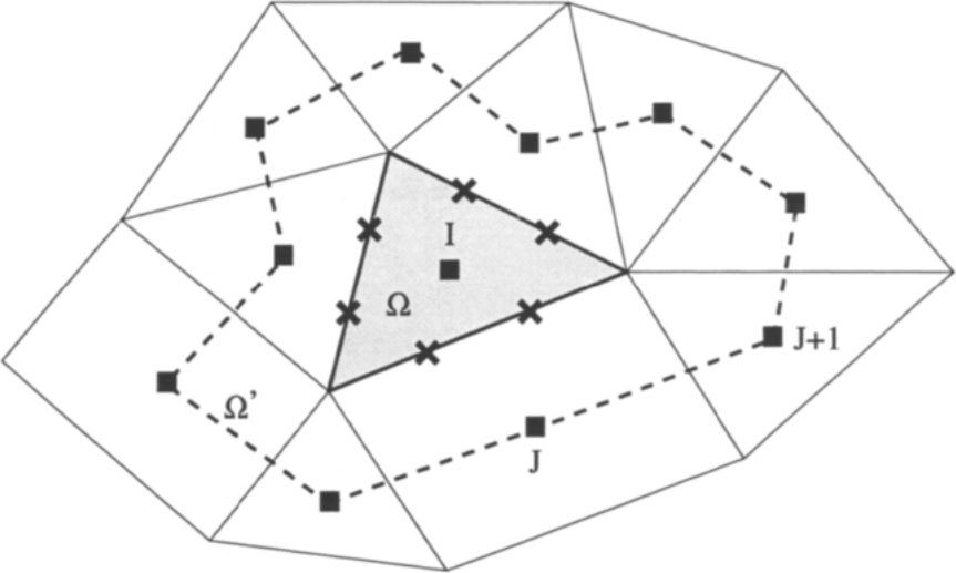
图5.14:Delanaye[62]、[63]二次重构方法在二维下的模板(实心矩形)。图例:虚线表示Green-Gauss梯度计算的积分路径(控制体\(\Omega'\));叉号表示通量积分的求积点;\(I\)、\(\Omega\)——中心单元及其控制体;\(J\)、\(J+1\)——模板中的远邻单元形心。