5.2 General Discretisation Methodologies 一般离散化方法[cfd-5-2]
我们在本章开头已经提到ï¼在控制体的定义和流动变量的布置方面有两种常用的做法:单元中心格式和中位对偶格式。本节将对两者作更详细的介绍。en
We already mentioned at the beginning of this chapter that there are two popular approaches for the definition of the control volume and for the location of the flow variables. These are the cell-centred scheme and the median-dual scheme. We shall present both in more detail in this section.
不过ï¼在开始之前ï¼先简要谈一谈非结构流动求解器所需的基本数据结构。事实上ï¼一个灵活而在内存和运算量方面又高效的数据结构ï¼是任何非结构格式的关键所在。可以说ï¼网格中所缺失的结构必须在求解器内部来提供。至少需要以下数据:
- 网格节点(顶点)的坐标;
- 从元素指向网格节点的指针;
- 从位于边界上的元素面指向网格节点的指针。
en
However, before we start, let us say a few words about the basic data structure which is needed for an unstructured flow solver. In fact, a flexible but in terms of memory and operation count efficient data structure is the crucial point of any unstructured scheme. You can say that the structure which is missing in the grid has to be provided inside the solver. At least the following data is required:
- coordinates of the grid nodes (vertices),
- pointers from elements to grid nodes,
- pointers from faces of elements located on a boundary to grid nodes.
离散格式所需的进一步数据结构可以由这些信息生成。为说明上述数据可能如何存储ï¼让我们以图5.4a中的四面体为例。如果进一步假设面1-2-4位于某一边界(壁面、入口、远场等)上ï¼则可以采用如下格式:en
Further data structures, which are required by the discretisation schemes, can be generated from this information. In order to illustrate how the above data could possibly be stored, let us consider for example the tetrahedron in Fig. 5.4a. If we further assume that the face 1-2-4 is on a boundary (wall, inlet, farfield, etc.), we could employ the format:
# nodes (x, y, z):
  P1.x  P1.y  P1.z
  P2.x  P2.y  P2.z
  P3.x  P3.y  P3.z
  P4.x  P4.y  P4.z
  ...
# tetrahedra:
  ...
  P1  P2  P3  P4
  ...
# boundaries:
  ...
  type  P1  P4  P2
  ...
随书CD-ROM所附的二维非结构代码也采用类似的格式。en
A similar format is also utilised by the 2-D unstructured code provided on the accompanying CD-ROM.
关于计算域的边界ï¼认识到以下两点十分重要。第一ï¼存储边界面比只存储(边界)节点更为方便。考察图5.5所示的情景即可理解这一点。问题在于:节点\(P_1\)被三条边界共享ï¼节点\(P_2\)和\(P_3\)被两条物理类型可能不同的边界共享。因此ï¼施加正确的边界条件可能变得非常繁琐。相反ï¼一个面只能属于一条边界ï¼例如\(P_1-P_2-P_4\)属于边界1。en
It is important to realise the following two points related to the boundaries of the computational domain. First, it is more convenient to store boundary faces than just the nodes. This can be understood by considering the situation depicted in Fig. 5.5. The problem is that node \(P_1\) is shared by three, nodes \(P_2\) and \(P_3\) by two boundaries of possibly physically different types. Therefore, it can become very cumbersome to apply the correct boundary conditions. On the contrary, a face can belong to only one boundary, like \(P_1-P_2-P_4\) to boundary 1.
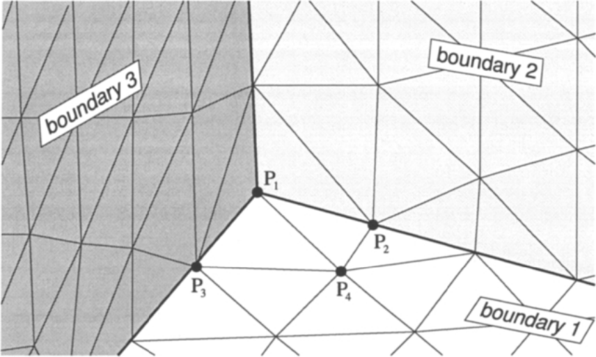
图5.5:相交于一个角点的三条边界——网格点相对于边界类型的二义性(ambiguity)。图例:三条边界分别标记为boundary 3、boundary 2、boundary 1;节点\(P_1\)、\(P_2\)、\(P_3\)位于边界交汇处附近,\(P_4\)为相邻内部节点;面\(P_1-P_2-P_4\)属于边界1。
5.2.1 Cell-Centred Scheme 单元中心格式[cfd-5-2-1]
如果控制体与网格单元完全相同ï¼且流动变量布置在各单元的形心处(如图5.6所示)ï¼我们就称之为单元中心格式。在计算离散化流动方程(5.2)时ï¼需要在控制体各面的中点处提供对流通量和黏性通量ï¼这对光滑网格上的二阶精度离散化已经足够(四边形面采用平均法向量)。通量可以用以下三种方式之一来近似:
- 通量平均(average of fluxes):由单元面左右两侧网格单元形心处之值分别计算通量ï¼再取平均ï¼但使用同一单位法向量(一般只用于对流通量);
- 变量平均(average of variables):采用单元面左右两侧相邻网格单元形心处变量的平均;
- 由周围单元之值分别在单元面两侧重构(reconstructed)流动量ï¼再由此计算通量(只用于对流通量)。
en
We speak of a cell-centred scheme if the control volumes are identical with the grid cells and if the flow variables are associated with their centroids, as it is sketched in Fig. 5.6. When we evaluate the discretised flow equations (5.2), we have to supply the convective and the viscous fluxes at the midpoints of the faces of the control volume, which is sufficient for a second-order accurate discretisation on smooth grids (averaged normal vector is employed for quadrilateral faces). The fluxes can be approximated in one of three ways:
- by the average of fluxes computed from values at the centroids of the grid cells to the left and to the right of the cell face, but using the same unit normal vector (generally applied only to the convective fluxes);
- by using an average of variables associated with the centroids of the grid cells adjacent to the left and to the right side of the cell face;
- by computing the fluxes from flow quantities reconstructed separately on both sides of the cell face from values in the surrounding cells (employed only for the convective fluxes).
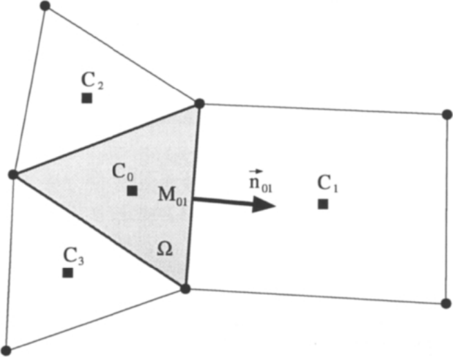
图5.6:单元中心格式的控制体(二维)。图例:网格节点用圆点表示ï¼单元中心用方块(C)表示;\(C_0\)、\(C_1\)、\(C_2\)、\(C_3\)为相邻单元的形心,\(M_{01}\)为面01的中点,\(\vec{n}_{01}\)为面01的单位法向量,\(\Omega\)为控制体(阴影部分)。
于是ï¼以图5.6中具有单位法向量\(\vec{n}_{01}\)的单元面为例ï¼第一种方法——通量平均——在二维情形下为en
Thus, considering for example the cell face with the unit normal vector \(\vec{n}_{01}\) in Fig. 5.6, the first approach - average of fluxes - reads in two dimensions
第二种方法——变量平均——可以表述为en
The second approach - average of variables - can be formulated as follows
其中在具有单位法向量\(\vec{n}_{01}\)的面上的守恒变量/因变量ï¼定义为两个相邻单元处数值的算术平均ï¼即en
where the conservative/dependent variables at the face with the unit normal vector \(\vec{n}_{01}\) are defined as the arithmetic average of values at the two adjacent cells. Thus,
第三种方法首先把流动量(通常为速度分量、压力、密度和总焓)分别插值到单元面的两侧。重构得到的量——称为左状态(left)和右状态(right state)(参见5.3.3小节)——一般并不相同。随后ï¼利用适当的非线性函数ï¼由左、右状态之差计算通过单元面的通量ï¼即en
The third methodology starts with an interpolation of flow quantities (usually velocity components, pressure, density and total enthalpy) separately to both sides of the cell face. The reconstructed quantities - termed the left and the right state (see Subsection 5.3.3) - differ in general. The fluxes through the cell face are then evaluated from the difference of the left and right state using an appropriate non-linear function. Hence,
其中en
where
它们表示重构得到的(左、右)状态。en
represent the reconstructed states.
正如本节开头所指出的ï¼描述元素的基本数据结构必须以适当的方式加以扩展ï¼以支持相应的离散化方法。从上面的讨论可以清楚地看出ï¼数值运算主要是利用元素(控制体)的面以及相邻单元中心处的值来进行的。因此ï¼很自然地应在空间离散化中采用基于面(face-based)的数据结构。这种数据结构对网格中每个具体的面(见图5.6)存储:
- 指向共享该面的两个单元的指针——借此可以访问与这两个单元(\(C_0\)、\(C_1\))相关联的流动变量;
- 面向量(\(\vec{S}_{01} = \vec{n}_{01}\Delta S_{01}\))——必须一致地指向外侧或内侧;
- 从各单元形心指向面中点\(M_{01}\)的两个向量ï¼即(\(C_0-M_{01}\))、(\(C_1-M_{01}\))——把流动变量精确插值到面上时需要。对纯四面体网格无需此项ï¼此时可用简单的外插公式[26]、[2](参见方程(5.44))。
en
As we already stated in the introduction to this section, the basic data structure which describes the elements has to be extended in an appropriate way to support the discretisation methodology. It is obvious from the previous discussion that numerical operations are carried out using mainly the faces of the elements (control volumes) together with values at the centres of the adjacent cells. It is therefore quite natural to employ a face-based data structure for the spatial discretisation. Such data structure stores for each particular face in the grid (see Fig. 5.6):
- pointers to the two cells which share the respective face - this allows us to access the flow variables associated with the two cells (\(C_0\), \(C_1\));
- the face vector (\(\vec{S}_{01} = \vec{n}_{01}\Delta S_{01}\)) - must point consistently either outwards or inwards;
- two vectors from the centroid each cell to the midpoint of the face \(M_{01}\), i.e., (\(C_0-M_{01}\)), (\(C_1-M_{01}\)) - required for an accurate interpolation of flow variables to the face. This is not necessary for purely tetrahedral grids, where a simple extrapolation formula can be used [26], [2] (cf. Eq. (5.44)).
DO face = 1, nfaces
    I = pointer_to_left_cell( face )
    J = pointer_to_right_cell( face )
    (F dS)_IJ = F(W_IJ, n_IJ) dS_IJ   (approx.)
    R_I = R_I + (F dS)_IJ
    R_J = R_J - (F dS)_IJ
ENDDO
循环结束后ï¼再加上源项\(\vec{Q}_I\Omega_I\)ï¼就得到所有单元内的最终残差(\(\vec{R}\))。效率较低的替代做法是对元素作循环ï¼因为这样面向量必须存储两次ï¼且通量要计算两次(边界除外)。此外ï¼由于我们使用完全相同的面向量\(\vec{S}_{IJ}\)来计算流入体积\(\Omega_I\)和\(\Omega_J\)的部分通量ï¼控制方程的守恒性质自动得以保持。en
After the loop is completed and the source term \(\vec{Q}_I\Omega_I\) is added, we obtain the final residuals (\(\vec{R}\)) in all cells. A less efficient approach would be to loop over elements because the face vectors would have to be stored twice and the fluxes would be computed twice (with the exception of the boundaries). Furthermore, because we use exactly the same face vector \(\vec{S}_{IJ}\) in order to to evaluate the partial fluxes into the volumes \(\Omega_I\) and \(\Omega_J\), the conservation properties of the governing equations are automatically retained.
5.2.2 Median-Dual Cell-Vertex Scheme 中位对偶单元顶点格式[cfd-5-2-2]
在单元顶点格式中ï¼流动变量与网格节点(顶点)相关联。中位对偶控制体通过连接共享该节点的所有单元的形心、面中点和边中点而构成。图5.7a给出了四面体的情形ï¼图5.7b给出了六面体的情形。中位对偶控制体的定义在每个网格节点周围形成一个多面体外壳ï¼如图5.8所示的二维混合网格情形。这些多面体可以看作一幅对偶网格(dual grid)——这正是该格式名称的由来。有趣的是ï¼中位对偶有限体积离散化等价于采用线性元素的Galerkin有限元格式(参见例如[36])。en
Within the cell-vertex scheme, the flow variables are associated with the grid nodes (vertices). Median-dual control volumes are formed by connecting the centroids, face- and edge-midpoints of all cells sharing the particular node. This is depicted in Fig. 5.7a for a tetrahedron and in Fig. 5.7b for a hexahedron. The definition of a median-dual control volume results in a polyhedral hull around each grid node, as it is sketched in Fig. 5.8 for a 2-D mixed grid. This polyhedra can be viewed as a dual grid - hence the name of the scheme. It is interesting to note that the median-dual finite volume discretisation is equivalent to the Galerkin finite element scheme with linear elements (see, e.g., [36]).
为了计算离散化流动方程(5.2)ï¼必须把对流通量和黏性通量在控制体表面上积分。因此ï¼严格来说需要对每个部分面(例如图5.7a中的\(F_1-M_{13}-F_2-C\))分别计算通量。然而ï¼只有三阶或更高阶精度的离散化才需要这样做[37]、[38]。对最常用的二阶格式ï¼可以假设流动变量在围绕某条边分组的所有面上为常数ï¼然后在边的中点处ï¼利用来自两个节点的变量和梯度计算通量。这一做法使我们能为每条边定义一个平均单位法向量和一个总面面积。于是ï¼参照图5.8ï¼例如边\(P_0-P_1\)的平均法向量为en
In order to evaluate the discretised flow equations (5.2), we have to integrate the convective and viscous fluxes over the surface of the control volume. Hence, we would have to compute the fluxes for each partial face (e.g., \(F_1-M_{13}-F_2-C\) in Fig. 5.7a) separately. However, this is only required for a third- or higher-order accurate discretisations [37], [38]. In the case of a second-order scheme, which is most frequently employed, we may assume the flow variables to be constant for all faces grouped around a particular edge. The fluxes are then evaluated at the midpoint of the edge using the variables and the gradients from both nodes. This approach allows us to define a mean unit normal vector and a total face area associated with each edge. Thus referring to Fig. 5.8, the mean normal vector, e.g., for the edge \(P_0-P_1\) becomes
而总面面积为\(\Delta S_{01} = \Delta S_L + \Delta S_R\)。同样的做法也适用于三维情形:平均法向量由共享该边中点的所有部分面求和得到ï¼如图5.9所示。面向量(\(\vec{S} = \vec{n}\Delta S\))在二维由方程(5.6)计算。在三维ï¼部分面总是四边形ï¼既可以把它们分成三角形后用方程(5.11)ï¼也可以采用基于方程(5.13)的简化处理ï¼后者对光滑网格已经足够。元素形心和面中心分别由公式(5.17)、(5.8)或(5.9)得到。en
and the total face area is given by: \(\Delta S_{01} = \Delta S_L + \Delta S_R\). The same applies also in 3D, where the mean normal vector results from a sum over all partial faces having the particular edge-midpoint in common, as it is rendered in Fig. 5.9. The face vector (\(\vec{S} = \vec{n}\Delta S\)) is computed in 2D from Eq. (5.6). In three dimensions, where the partial faces are always quadrilaterals, we can either divide them into triangles and use Eq. (5.11), or we can employ a simplified treatment due to Eq. (5.13), which is sufficient for smooth grids. The element centroids and the face centres are obtained by the formulae (5.17), (5.8), or (5.9), respectively.
然后ï¼通量可以按以下三种方法之一计算:
- 通量平均:由一条边两个节点处之值分别计算通量ï¼再取平均ï¼但使用同一平均单位法向量(一般只用于对流通量);
- 变量平均:采用存储在一条边两个节点处的变量的平均;
- 由周围节点之值分别在控制体面两侧重构(reconstructed)流动量ï¼再由此计算通量(只用于对流通量)。
en
The fluxes can then be evaluated according to one of the three following methodologies:
- by the average of fluxes computed from values at both nodes of an edge, but using the same mean unit normal vector (generally applied only to the convective fluxes);
- by using an average of variables stored at the two nodes of an edge;
- by computing the fluxes from flow quantities reconstructed separately on both sides of the face of the control volume from values at the surrounding nodes (employed only for the convective fluxes).
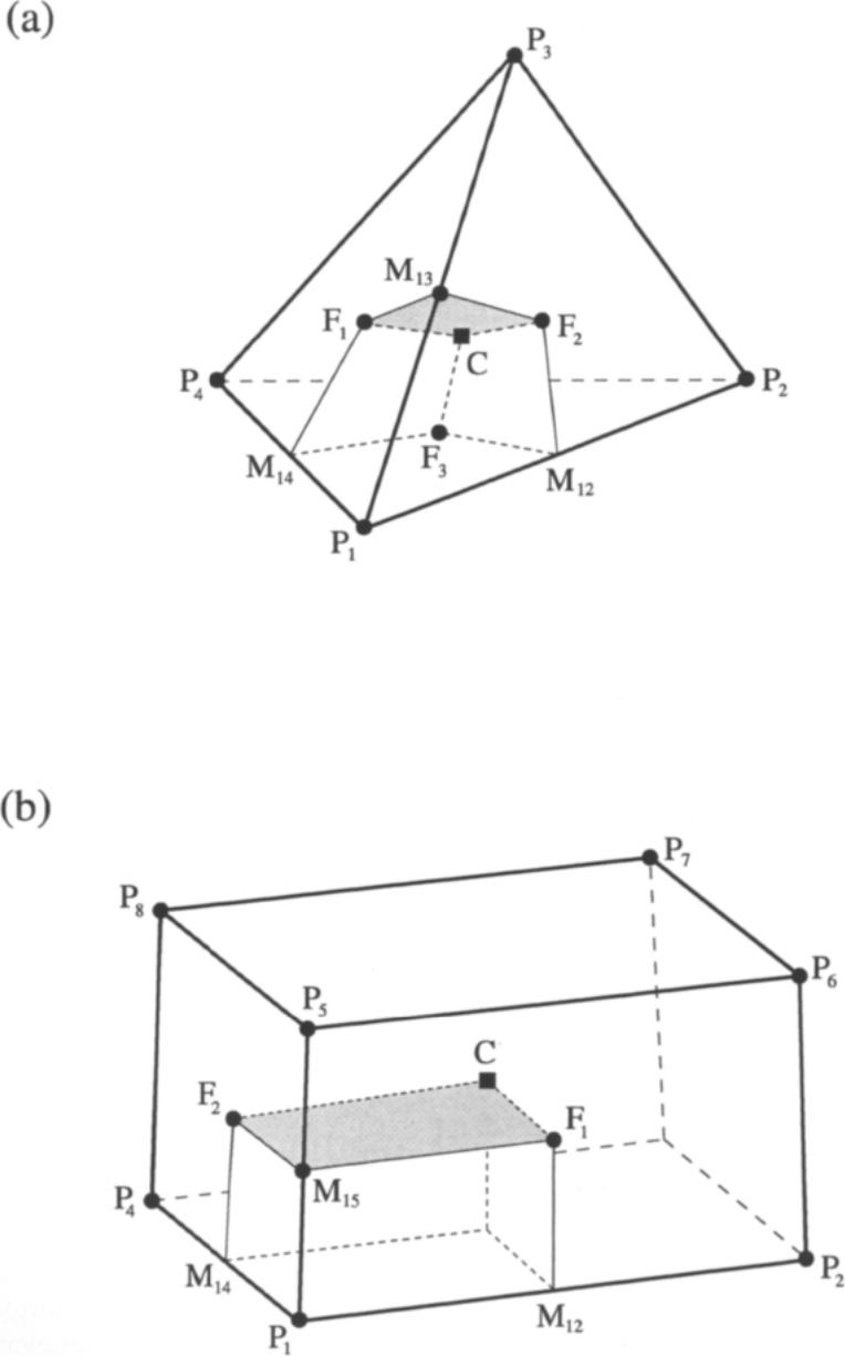
图5.7:四面体(a)与六面体(b)的中位对偶格式的部分控制体及面(阴影所示)。P表示网格节点,C为单元形心(方程(5.17)),F为面形心(方程(5.8)或(5.9)),M表示边中点。阴影部分表示分配给边\(P_1-P_3\)或\(P_1-P_5\)的控制体面的一部分。
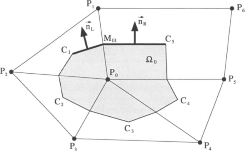
图5.8:中位对偶格式的控制体(二维)。\(C_1\)、\(C_2\)等表示单元中心(形心);\(P_1\)、\(P_2\)等表示网格节点。与边\(P_0-P_1\)相关联的面面积用粗线标出。图中还标出了部分面的单位法向量\(\vec{n}_L\)、\(\vec{n}_R\)ï¼边\(P_0-P_1\)的中点\(M_{01}\)ï¼以及网格节点\(P_0\)周围的控制体\(\Omega_0\)。
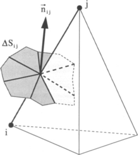
图5.9:三维中位对偶单元顶点格式中与边\(ij\)相关联的总面面积\(\Delta S_{ij}\)与平均单位法向量\(\vec{n}_{ij}\)。
通量的计算在形式上与单元中心格式所用的方法相同ï¼因此公式(5.18)-(5.22)在中位对偶格式中同样适用。如果采用上面这种把每条边与一个平均单位法向量相关联的做法ï¼那么最有效率的方法是在空间离散化中采用基于边(edge-based)的数据结构。这种数据结构对网格中每条具体的边(参见图5.9)存储:
- 指向定义该边的两个节点的指针——借此可以访问与两个控制体\(\Omega_i\)和\(\Omega_j\)相关联的流动变量;
- 面向量(\(\vec{S}_{ij} = \vec{n}_{ij}\Delta S_{ij}\))——必须一致地指向外侧或内侧;
- 从节点\(i\)指向节点\(j\)的边向量——把流动变量插值到面上(解的重构)时需要。另一种做法是ï¼边向量可以由节点坐标即时算得。对于带人工耗散的标准中心格式(5.3.1小节)ï¼此项并不需要。
en
The computation of fluxes follows formally the same approaches as for the cell-centred scheme. Thus, the formulae (5.18)-(5.22) are applicable also in the case of the median-dual scheme. If we utilise the above approach which associates each edge with a mean unit normal, the most efficient methodology is to employ an edge-based data structure for the spatial discretisation. The edge-based data structure stores for each particular edge in the grid (cf. Fig. 5.9):
- pointers to the two nodes which define the edge - this allows us to access the flow variables associated with the two control volumes \(\Omega_i\) and \(\Omega_j\);
- the face vector (\(\vec{S}_{ij} = \vec{n}_{ij}\Delta S_{ij}\)) - must point consistently either outwards or inwards;
- the edge vector from node \(i\) to node \(j\) - required for the interpolation of flow variables to the face (solution reconstruction). Alternatively, the edge vector can be computed on the fly from coordinates of the nodes. This is not required for the standard central scheme with artificial dissipation (Subsection 5.3.1).
DO edge = 1, nedges
    i = pointer_to_left_node( edge )
    j = pointer_to_right_node( edge )
    (F dS)_ij = F(W_ij, n_ij) dS_ij   (approx.)
    R_i = R_i + (F dS)_ij
    R_j = R_j - (F dS)_ij
ENDDO
循环结束后ï¼再加上源项\(\vec{Q}_i\Omega_i\)ï¼就得到所有节点处的最终残差(\(\vec{R}\))。与对每个控制体分别累加通量相比ï¼这一方法的效率显著更高ï¼因为每个平均面向量只存储一次ï¼而且每条边也只访问一次而不是两次。此外ï¼由于我们使用完全相同的平均面向量\(\vec{S}_{ij}\)来计算流入体积\(\Omega_i\)和\(\Omega_j\)的部分通量ï¼质量、动量和能量严格保持守恒。en
After the loop is completed and the source term \(\vec{Q}_i\Omega_i\) is added, we obtain the final residuals (\(\vec{R}\)) in all nodes. This approach is significantly more efficient than summing up the fluxes over each control volume separately, because we store each mean face vector only once and we also visit each edge only once instead of twice. Furthermore, since we use exactly the same mean face vector \(\vec{S}_{ij}\) in order to to evaluate the partial fluxes into the volumes \(\Omega_i\) and \(\Omega_j\), the mass, momentum and energy remain exactly conserved.
5.2.3 Cell-Centred versus Median-Dual Scheme 单元中心格式与中位对偶格式的比较[cfd-5-2-3]
单元中心格式与中位对偶格式孰优孰劣ï¼一直是颇具争议的话题。主要原因在于ï¼缺少针对真实外形、在精度、计算时间和内存等方面对两种方法的公平比较。我们此处的意图ï¼是围绕以下四个方面收集支持与反对每种方法的最重要论据:
- 精度;
- 计算量;
- 内存需求;
- 灵活性。
en
The relative advantages and disadvantages of the cell-centred and the median-dual scheme are the subject of controversial debates. The main reason is the lack of fair comparisons of the two methodologies with respect to accuracy, computational time and memory for realistic configurations. Our intention here is to collect the most important arguments for and against each of the approaches regarding:
- accuracy,
- computational work,
- memory requirements, and
- flexibility.
这应有助于更深入地理解每种格式固有的问题ï¼并有助于针对具体的应用选择最合适的格式。en
This should lead to a greater understanding of the problems inherent to each scheme and should be of help in selecting the most suitable scheme for the intended applications.
Accuracy 精度
在三角形/四面体网格上ï¼单元中心格式得到的控制体数量(从而自由度)约为中位对偶格式的两倍/六倍[36]。在由四面体和棱柱构成的典型混合网格上ï¼单元中心格式给出的未知量数目约为中位对偶格式的三倍。这表明在相同网格上ï¼单元中心格式比单元顶点离散化更精确。然而ï¼与中位对偶格式相比ï¼单元中心格式的残差由少得多的通量累加而成(在四面体网格上约为三个对七个)ï¼这可能损害精度。因此ï¼究竟哪种格式更优ï¼并没有明确的证据。en
A cell-centred scheme on a triangular/tetrahedral grid leads to about twice/six times as many control volumes and hence degrees of freedom as a median-dual scheme [36]. On typical mixed grids, which consist of tetrahedra and prisms, a cell-centred scheme gives roughly three times more unknowns than a median-dual scheme. This suggests that cell-centred schemes are more accurate than cell-vertex discretisations on an identical grid. However, the residual of a cell-centred scheme results from a much smaller number of fluxes as compared to a median-dual scheme (three versus approximately seven on a tetrahedral grid), which may impair the accuracy. Thus, there is no clear evidence about which scheme might be superior.
中位对偶格式在拉伸的三角形和四面体网格上存在一个特有的问题。例如考虑图5.10ï¼它显示了由直角三角形组成的网格剖分ï¼这种剖分常用于黏性流动中的固体壁面附近。从图5.10a可以看到ï¼面\(\Delta S_{ij}\)相对于边\(ij\)变得高度倾斜。然而ï¼空间离散格式大多假设通量与面正交(尤其是黎曼求解器)。由此引入的误差对一阶格式尤为显著[38]。采用所谓的包含对偶(containment-dual)控制体[39]可以改善这一状况。如图5.11所示ï¼包含对偶方法用最小外包圆/球的中心代替单元形心来定义面。这样得到的控制体与四边形网格上的相同(图5.10b)。注意ï¼像\(ij'\)这样的对角边没有与之相关联的面面积。这需要额外的预处理工作量ï¼但解的精度可以得到明显改善[40]。当然ï¼另一种可能的做法是直接在(边界层内)采用四边形或六面体en
The median-dual scheme suffers from a particular problem on stretched triangular and tetrahedral grids. Consider, for example, Fig. 5.10, which shows a tessellation composed of right triangles, as it is often employed near solid walls for viscous flows. We can see in Fig. 5.10a that the face \(\Delta S_{ij}\) becomes highly skewed with respect to the edge \(ij\). However, spatial discretisation schemes mostly assume fluxes to be orthogonal to a face (especially Riemann solvers). Thus, an error is introduced which is particularly significant for a first-order scheme [38]. The situation can be improved using the so-called containment-dual control volume [39]. As depicted in Fig. 5.11, the containment-dual approach employs the centres of the minimum spanning circles/spheres instead of the cell centroids to define the faces. This leads to control volumes identical to those on quadrilateral grids (Fig. 5.10b). Notice that there is no face area associated with diagonal edges like \(ij'\). An additional effort is required for pre-processing, but the solution accuracy can be improved noticeably [40]. Of course, another possibility is to employ directly quadrilateral or hexahedral
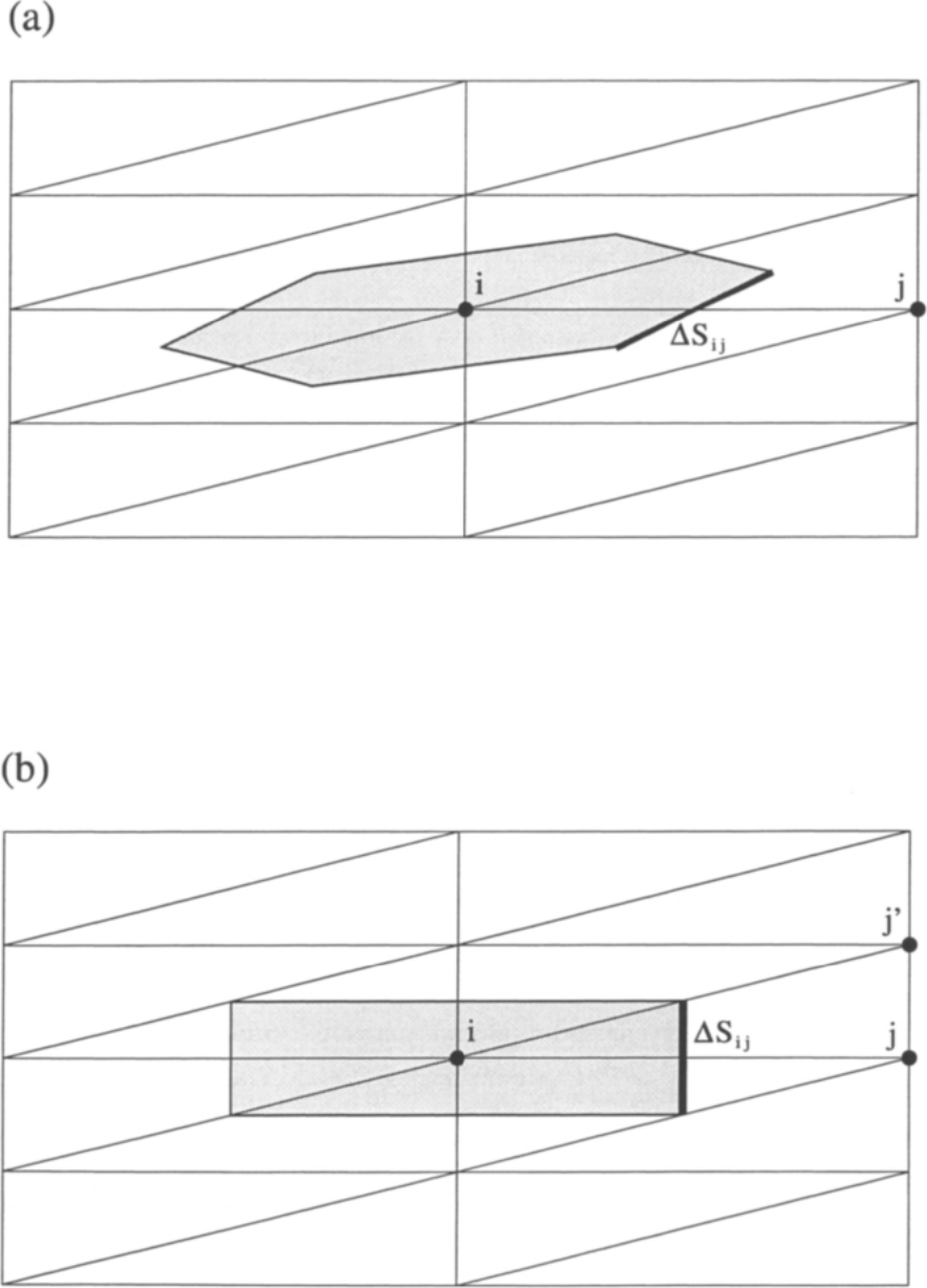
图5.10:对拉伸直角三角形剖分ï¼中位对偶(a)与包含对偶(b)控制体的比较。图例:阴影部分为控制体,\(i\)、\(j\)为节点,\(\Delta S_{ij}\)为与边\(ij\)相关联的(粗线所示)面;(b)中\(j'\)为包含对偶在最长边上引入的节点。
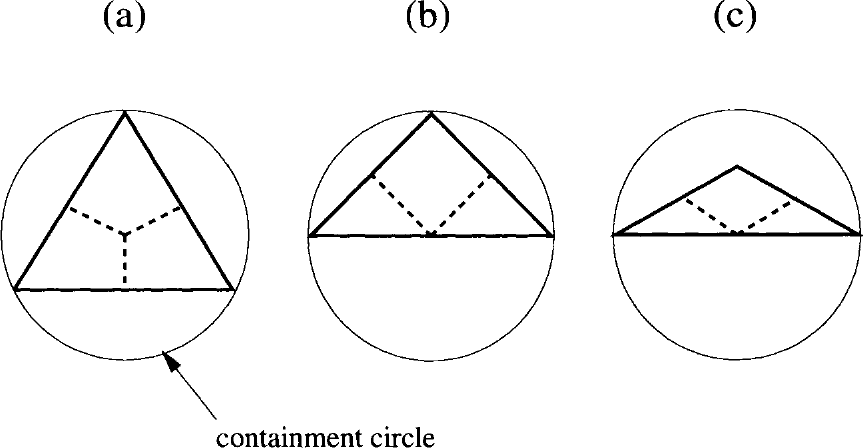
图5.11:锐角(a)与钝角(c)三角形情形下包含对偶(虚线)的一部分[40]。包含圆(containment circle)是包含该三角形的最小圆;对钝角三角形ï¼它的圆心位于最长边上。
(单元)。关于网格诱导误差的进一步讨论可参见文献[22]和[23]。en
cells within the boundary layers. Further discussion of grid-induced errors can be found in Ref. [22] and [23].
中位对偶格式固有的另一个问题ï¼出现在物理域边界处的离散化。具体而言ï¼在边界处只剩下大约半个控制体(参见图4.6)。围绕各面对通量积分ï¼得到的残差位于控制体内部(inside)——理想情况下在其中心(centre);然而ï¼残差却被关联到直接位于边界上的节点(node)。与单元中心格式相比ï¼这种失配导致离散化误差增大ï¼这在固体壁面上尤其不利。对偶控制体的定义还会在尖锐角点(如尾缘)处引起问题ï¼表现为压力或密度中的非物理峰值。在周期性边界处(参见第8.8章)还会出现进一步的复杂情况:必须把来自控制体两部分的通量正确地相加。en
Another problem inherent to the median-dual scheme is the discretisation at boundaries of the physical domain. What happens is that there is only about one half of the control volume left at the boundary (cf. Fig. 4.6). The integration of fluxes around the faces results in a residual located inside - ideally at the centre - of the control volume. However, the residual is associated with the node, residing directly on the boundary. This mismatch leads to increased discretisation error in comparison to the cell-centred scheme, which is particularly undesirable on solid walls. The definition of the dual control volume causes also problems at sharp corners (like trailing edges), which show up as unphysical peaks in pressure or density. Further complications arise at periodic boundaries (see Chapter 8.8), where the fluxes from both parts of the control volume have to be summed up correctly.
控制体形心与残差存储节点之间的失配ï¼对中位对偶格式还有进一步的影响:在非定常流动情形下ï¼它表现为质量矩阵。这一点我们在3.2节开头已经讨论过。单元中心格式的优点是ï¼可以在不牺牲解的精度的情况下从方程中消去质量矩阵;与此相反ï¼中位对偶格式需要对质量矩阵作特殊处理[41]、[42]。en
The mismatch between the centroid of the control volume and the node where the residual is stored has also a further implication for the median-dual scheme. It arises as the mass matrix in the case of unsteady flows. We discussed this point already at the beginning of Section 3.2. The advantage of the cell-centred scheme is that the mass matrix can be eliminated from the equations, without compromising the solution accuracy. By contrast, the median-dual scheme requires a special treatment of the mass matrix [41], [42].
Computational Work 计算量
要判断两种格式所需的计算量ï¼主要须考察通量的积分。从前面的讨论可知ï¼单元中心格式对单元面作循环ï¼而中位对偶格式对边作循环。由于两种格式在交界面上计算通量的方式相当类似ï¼单元面数与边数之比就给出了计算量之比。因此ï¼在四面体网格上ï¼单元面数(若每两个单元只计一次)约为边数的两倍ï¼因而在相同网格上ï¼单元中心格式的计算代价约为中位对偶格式的两倍[36]。然而ï¼在含棱柱单元的混合网格上ï¼单元中心方法变得更有竞争力。在六面体网格上ï¼面数等于边数ï¼除边界处理外ï¼两种方法的计算量相当。en
In order to judge the computational effort required for both schemes, we have to consider primarily the integration of the fluxes. We know from the previous discussion that the cell-centred scheme uses a loop over cell faces whereas the median-dual scheme loops over the edges. Since the evaluation of the fluxes at an interface is quite similar for both schemes, the ratio of the number of cell faces to the number of edges gives the ratio of the computational work. Thus, on a tetrahedral grid, where the number cell faces (if counted only once for every two cells) is approximately two times larger than the number of edges, the cell-centred scheme is computationally twice as much expensive as the median-dual scheme on an identical grid [36]. The cell-centred approach becomes however more competitive on mixed grids containing prismatic elements. Apart from boundary treatment, both methods are computationally equivalent on hexahedral grids, where the number of faces equals the number of edges.
Memory Requirements 内存需求
就内存需求而言ï¼与中位对偶格式相比ï¼单元中心格式在四面体网格上需要存储的流动变量约为其六倍ï¼在通常的混合网格上约为其三倍。此外ï¼如前所述ï¼两种格式都需要为每个单元面或每条边分别存储两个整数和三个实数(指针与面向量)。另外ï¼单元中心格式还必须在内存中为每个单元面保存两个指向面中点的向量——6个实数。相反ï¼中位对偶格式只依靠节点坐标即可工作ï¼所需数值要少得多。总而言之ï¼平均来说ï¼单元中心格式所需的计算机内存是中位对偶方法的两倍以上。en
Considering the memory requirements, the cell-centred scheme has to store about six times more flow variables on tetrahedral and about three times more variables on usual mixed grids as compared to the median-dual scheme. Furthermore, as we saw, both schemes require to store two integers and three reals (pointers and face vector) per cell face or edge, respectively. Additionally, the cell-centred scheme has to keep two vectors to the face-midpoint - 6 reals - per cell face in memory. On the contrary, the median-dual scheme can work with the node coordinates only, which are considerably fewer values. Thus in summary, the cell-centred scheme needs, on average, more than twice as much computer memory as the median-dual method.
Grid Generation/Adaptation 网格生成/自适应
单元中心格式的一个显著优势出现在非相容(non-conforming)单元界面的情形ï¼例如图3.4中字母“F”处的界面。与中位对偶方法不同ï¼在这种界面上计算通量不需要特殊而昂贵的处理。这使网格生成和网格自适应的灵活性得以提高。en
One significant advantage of the cell-centred scheme appears in the case of non-conforming cell interfaces, like those at the letter "F" in Fig. 3.4. In contrast to the median-dual methodology, no special and expensive procedure is required for the computation of the fluxes at the interface. This allows for an increased flexibility in the grid generation and also in the grid adaptation.