5.1.2 Three-Dimensional Case 三维情形[cfd-5-1-2]

与前面的二维情形不同ï¼在三维情形ï¼对具有四边形面的元素或控制体计算面向量和体积会遇到一些问题。主要原因在于ï¼控制体四边形面的四个顶点一般不一定位于同一平面内。此时ï¼法向量在这样的面上不再是常数(见图4.2)。为克服这一困难ï¼可以把每个四边形面分解成两个甚至更多的三角形。然而ï¼对光滑网格上的二阶格式而言ï¼精度上的收益几乎察觉不到。这种额外的代价只有对三阶及更高阶空间离散化才是值得的——实际上也是必需的。因此ï¼在下面的讨论中ï¼我们将对四边形面采用一种基于平均法向量的简化处理方法。en

As opposed to the previous 2-D case, the computation of face vectors and volumes poses in 3D some problems for elements or control volumes with quadrilateral faces. The main reason for this is that, in general, the four vertices of a quadrilateral face of a control volume may not lie in a plane. Then, the normal vector is no longer constant on such face (see Fig. 4.2). In order to overcome this difficulty, we could decompose each quadrilateral face into two or even more triangles. However, the gain in accuracy is hardly noticeable for a second-order scheme on a smooth grid. The additional effort can only be justified - and in fact it becomes necessary - for a third- and higher order spatial discretisations. Therefore, we shall apply a simplified treatment of the quadrilateral faces in the following considerations, which is based on an averaged normal vector.

Triangular face 三角形面

对于三角形面ï¼面向量 $\vec{S}$ 可以用高斯公式精确计算。按图5.4a定义节点ï¼对三角形1-2-3的边差分得到en

The face vector $\vec{S}$ can be exactly computed for a triangular face using Gauss' formula. Defining the nodes according to Fig. 5.4a, we obtain for the edge differences of the triangle 1-2-3

\begin{aligned} \Delta xy_A &= (x_1 - x_2)(y_1 + y_2), &\quad \Delta yz_A &= (y_1 - y_2)(z_1 + z_2),\\ \Delta xy_B &= (x_2 - x_3)(y_2 + y_3), &\quad \Delta yz_B &= (y_2 - y_3)(z_2 + z_3),\\ \Delta xy_C &= (x_3 - x_1)(y_3 + y_1), &\quad \Delta yz_C &= (y_3 - y_1)(z_3 + z_1),\\ \Delta zx_A &= (z_1 - z_2)(x_1 + x_2),\\ \Delta zx_B &= (z_2 - z_3)(x_2 + x_3),\\ \Delta zx_C &= (z_3 - z_1)(x_3 + x_1). \end{aligned} \tag{5.10}

于是ï¼外指面向量 $\vec{S} = \vec{n}\Delta S$ 由下式得到en

The outward pointing face vector $\vec{S} = \vec{n}\Delta S$ results then from

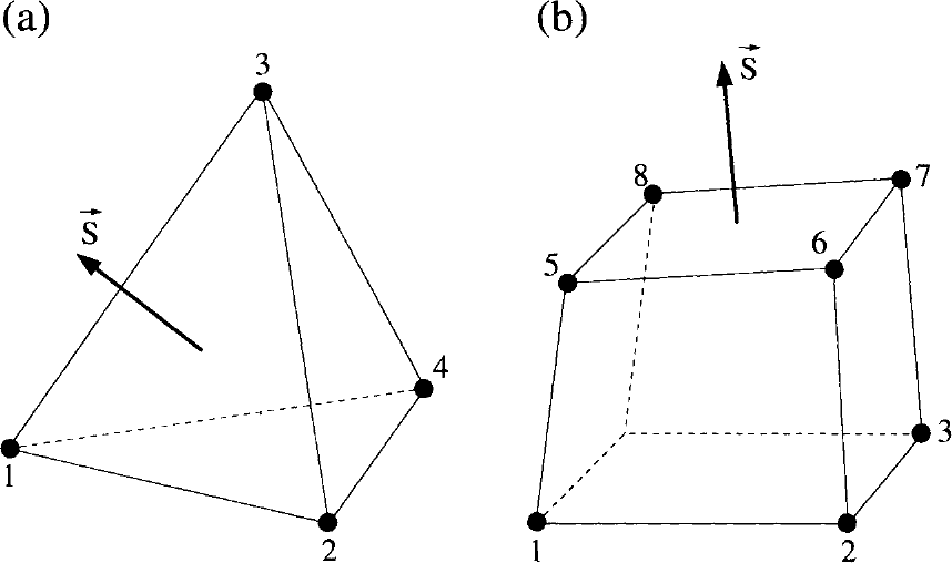
\vec{S} = \frac{1}{2}\begin{bmatrix} \Delta yz_A + \Delta yz_B + \Delta yz_C \\ \Delta zx_A + \Delta zx_B + \Delta zx_C \\ \Delta xy_A + \Delta xy_B + \Delta xy_C \end{bmatrix}. \tag{5.11}

图5.4:(a)四面体元素与(b)六面体元素的节点编号及面向量

图5.4:节点编号与面向量:(a)四面体元素;(b)六面体元素。图例:(a)中节点1—4为四面体的顶点, $\vec{S}$ 为面向量;(b)中节点1—8为六面体的顶点, $\vec{S}$ 为面5-6-7-8上的外指面向量。

Quadrilateral face 四边形面

四边形面(诸如图5.4b所示的面)的平均面向量 $\vec{S}$ ï¼最方便是采用与二维情形计算四边形面积相同的高斯公式来计算。于是ï¼对于图5.4b中由节点5、6、7和8给出的面ï¼首先定义如下差分en

The averaged face vector $\vec{S}$ of a quadrilateral face, like that rendered in Fig. 5.4b, is most conveniently computed using the same Gauss' formula as employed in 2-D for the area of a quadrilateral. Thus, for the face given by the nodes 5, 6, 7 and 8 in Fig. 5.4b, we first define the differences

\begin{aligned} \Delta x_A &= x_8 - x_6, &\quad \Delta x_B &= x_7 - x_5,\\ \Delta y_A &= y_8 - y_6, &\quad \Delta y_B &= y_7 - y_5,\\ \Delta z_A &= z_8 - z_6, &\quad \Delta z_B &= z_7 - z_5. \end{aligned} \tag{5.12}

然后ï¼由下述关系式得到外指面向量 $\vec{S} = \vec{n}\Delta S$ en

Then, we obtain the outward pointing face vector $\vec{S} = \vec{n}\Delta S$ from the relation

\vec{S} = \frac{1}{2}\begin{bmatrix} \Delta z_A\,\Delta y_B - \Delta y_A\,\Delta z_B \\ \Delta x_A\,\Delta z_B - \Delta z_A\,\Delta x_B \\ \Delta y_A\,\Delta x_B - \Delta x_A\,\Delta y_B \end{bmatrix}. \tag{5.13}

当面接近平行四边形ï¼即面的四个顶点全部位于同一平面内时ï¼这一近似变为精确的。en

The approximation becomes exact when the face approaches a parallelogram, i.e., when the vertices of the face lie all in one plane.

两种情形下的单位法向量都由 $\vec{n} = \vec{S}/\Delta S$ 得到ï¼其中en

The unit normal vector is obtained in both cases from $\vec{n} = \vec{S}/\Delta S$ with

\Delta S = \sqrt{S_x^2 + S_y^2 + S_z^2}, \tag{5.14}

其中 $$S_x$$ 、 $$S_y$$ 和 $$S_z$$ 分别表示由方程(5.11)或方程(5.13)给出的面向量的笛卡尔分量。en

where $$S_x$$ , $$S_y$$ and $$S_z$$ denote the Cartesian components of the face vector given by Eq. (5.11) or Eq. (5.13), respectively.

Volume 体积

正如在三维结构网格有限体积格式的情形中已经指出的ï¼体积的一种非常方便的计算方法基于散度定理(divergence theorem)[35]。4.1.2小节的讨论最终给出表达式en

As we already stated in the case of 3-D structured finite volume schemes, a very convenient approach for the computation of volumes is based on the divergence theorem [35]. The discussion in Subsection 4.1.2 led finally to the expression

\Omega = \frac{1}{3}\sum_{m=1}^{N_F}\left(\vec{r}_c\cdot\vec{S}\right)_m \tag{5.15}

此即体积的表达式ï¼其中 $$N_F$$ 表示控制体的面数, $(\vec{r}_c)_m$ 为控制体第 $$m$$ 个面的中心, $\vec{S}_m$ 为第 $$m$$ 个面(外指)的面向量。公式(5.15)可直接应用于非结构网格。对于所有面均为三角形、或四边形面均为平面的体积ï¼该公式是精确的。en

for the volume, where $$N_F$$ denotes the number of the faces of the control volume, $(\vec{r}_c)_m$ the centre of the face $$m$$ of the control volume, and $\vec{S}_m$ the face vector (outward directed) of the face $$m$$ , respectively. The formula (5.15) is directly applicable on unstructured grids. It is exact for a volume with triangular faces, or a volume with planar quadrilateral faces.

Cell Centroid 单元形心

前面提到的中位对偶型控制体需要知道网格单元的形心。一般体积的形心定义为en

The previously mentioned median-dual type of control volume requires the knowledge of the centroid of the grid cell. The centroid of a general volume is defined as

\vec{r}_c = \frac{1}{\Omega}\int_{\Omega}\vec{r}\,d\Omega\,. \tag{5.16}

根据文献[34]中的推导ï¼方程(5.16)的关系可以离散化为en

According to the derivation in Ref. [34], the relation in Eq. (5.16) can be discretised as

\vec{r}_c = \frac{3\sum\limits_{m=1}^{N_F}\left(\vec{r}_c\cdot\vec{n}\right)_m\left(\vec{r}_c\right)_m\Delta S_m}{4\sum\limits_{m=1}^{N_F}\left(\vec{r}_c\cdot\vec{n}\right)_m\Delta S_m}, \tag{5.17}

其中面 $$m$$ 的中心ï¼即 $(\vec{r}_c)_m$ ï¼对三角形面由方程(5.8)得到ï¼对四边形面由方程(5.9)得到。可以注意到ï¼方程(5.17)中的分母与方程(5.15)中的 $\Omega/3$ 相同。en

where the centre of a face $$m$$ , i.e., $(\vec{r}_c)_m$ is obtained from Eq. (5.8) for a triangular face, or from Eq. (5.9) for a quadrilateral face. As we can note, the denominator in Eq. (5.17) is identical to $\Omega/3$ from Eq. (5.15).