5.2.2 Median-Dual Cell-Vertex Scheme 中位对偶单元顶点格式[cfd-5-2-2]

在单元顶点格式中ï¼流动变量与网格节点(顶点)相关联。中位对偶控制体通过连接共享该节点的所有单元的形心、面中点和边中点而构成。图5.7a给出了四面体的情形ï¼图5.7b给出了六面体的情形。中位对偶控制体的定义在每个网格节点周围形成一个多面体外壳ï¼如图5.8所示的二维混合网格情形。这些多面体可以看作一幅对偶网格(dual grid)——这正是该格式名称的由来。有趣的是ï¼中位对偶有限体积离散化等价于采用线性元素的Galerkin有限元格式(参见例如[36])。en

Within the cell-vertex scheme, the flow variables are associated with the grid nodes (vertices). Median-dual control volumes are formed by connecting the centroids, face- and edge-midpoints of all cells sharing the particular node. This is depicted in Fig. 5.7a for a tetrahedron and in Fig. 5.7b for a hexahedron. The definition of a median-dual control volume results in a polyhedral hull around each grid node, as it is sketched in Fig. 5.8 for a 2-D mixed grid. This polyhedra can be viewed as a dual grid - hence the name of the scheme. It is interesting to note that the median-dual finite volume discretisation is equivalent to the Galerkin finite element scheme with linear elements (see, e.g., [36]).

为了计算离散化流动方程(5.2)ï¼必须把对流通量和黏性通量在控制体表面上积分。因此ï¼严格来说需要对每个部分面(例如图5.7a中的 $F_1-M_{13}-F_2-C$ )分别计算通量。然而ï¼只有三阶或更高阶精度的离散化才需要这样做[37]、[38]。对最常用的二阶格式ï¼可以假设流动变量在围绕某条边分组的所有面上为常数ï¼然后在边的中点处ï¼利用来自两个节点的变量和梯度计算通量。这一做法使我们能为每条边定义一个平均单位法向量和一个总面面积。于是ï¼参照图5.8ï¼例如边 $$P_0-P_1$$ 的平均法向量为en

In order to evaluate the discretised flow equations (5.2), we have to integrate the convective and viscous fluxes over the surface of the control volume. Hence, we would have to compute the fluxes for each partial face (e.g., $F_1-M_{13}-F_2-C$ in Fig. 5.7a) separately. However, this is only required for a third- or higher-order accurate discretisations [37], [38]. In the case of a second-order scheme, which is most frequently employed, we may assume the flow variables to be constant for all faces grouped around a particular edge. The fluxes are then evaluated at the midpoint of the edge using the variables and the gradients from both nodes. This approach allows us to define a mean unit normal vector and a total face area associated with each edge. Thus referring to Fig. 5.8, the mean normal vector, e.g., for the edge $$P_0-P_1$$ becomes

\vec{n}_{01} = \vec{n}_L + \vec{n}_R, \tag{5.23}

而总面面积为 $\Delta S_{01} = \Delta S_L + \Delta S_R$ 。同样的做法也适用于三维情形:平均法向量由共享该边中点的所有部分面求和得到ï¼如图5.9所示。面向量( $\vec{S} = \vec{n}\Delta S$ )在二维由方程(5.6)计算。在三维ï¼部分面总是四边形ï¼既可以把它们分成三角形后用方程(5.11)ï¼也可以采用基于方程(5.13)的简化处理ï¼后者对光滑网格已经足够。元素形心和面中心分别由公式(5.17)、(5.8)或(5.9)得到。en

and the total face area is given by: $\Delta S_{01} = \Delta S_L + \Delta S_R$ . The same applies also in 3D, where the mean normal vector results from a sum over all partial faces having the particular edge-midpoint in common, as it is rendered in Fig. 5.9. The face vector ( $\vec{S} = \vec{n}\Delta S$ ) is computed in 2D from Eq. (5.6). In three dimensions, where the partial faces are always quadrilaterals, we can either divide them into triangles and use Eq. (5.11), or we can employ a simplified treatment due to Eq. (5.13), which is sufficient for smooth grids. The element centroids and the face centres are obtained by the formulae (5.17), (5.8), or (5.9), respectively.

然后ï¼通量可以按以下三种方法之一计算:

通量平均:由一条边两个节点处之值分别计算通量ï¼再取平均ï¼但使用同一平均单位法向量(一般只用于对流通量);
变量平均:采用存储在一条边两个节点处的变量的平均;
由周围节点之值分别在控制体面两侧重构(reconstructed)流动量ï¼再由此计算通量(只用于对流通量)。

The fluxes can then be evaluated according to one of the three following methodologies:

by the average of fluxes computed from values at both nodes of an edge, but using the same mean unit normal vector (generally applied only to the convective fluxes);
by using an average of variables stored at the two nodes of an edge;
by computing the fluxes from flow quantities reconstructed separately on both sides of the face of the control volume from values at the surrounding nodes (employed only for the convective fluxes).

图5.7:四面体(a)与六面体(b)的中位对偶格式的部分控制体及面(阴影)

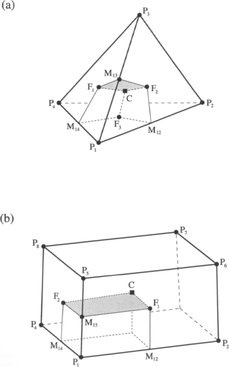
图5.7:四面体(a)与六面体(b)的中位对偶格式的部分控制体及面(阴影所示)。P表示网格节点,C为单元形心(方程(5.17)),F为面形心(方程(5.8)或(5.9)),M表示边中点。阴影部分表示分配给边 $$P_1-P_3$$ 或 $$P_1-P_5$$ 的控制体面的一部分。

图5.8:中位对偶格式的控制体(二维)

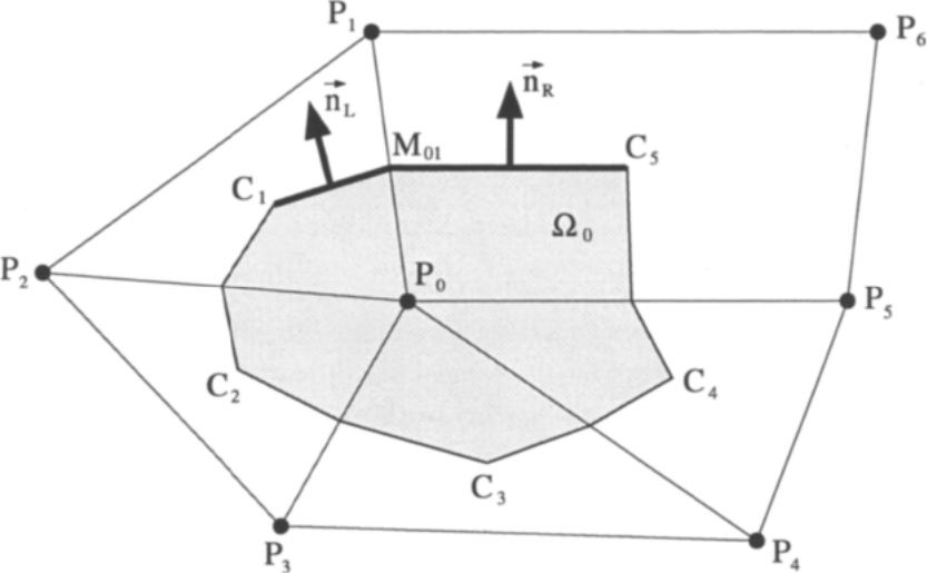
图5.8:中位对偶格式的控制体(二维)。 $$C_1$$ 、 $$C_2$$ 等表示单元中心(形心); $$P_1$$ 、 $$P_2$$ 等表示网格节点。与边 $$P_0-P_1$$ 相关联的面面积用粗线标出。图中还标出了部分面的单位法向量 $\vec{n}_L$ 、 $\vec{n}_R$ ï¼边 $$P_0-P_1$$ 的中点 $M_{01}$ ï¼以及网格节点 $$P_0$$ 周围的控制体 $\Omega_0$ 。

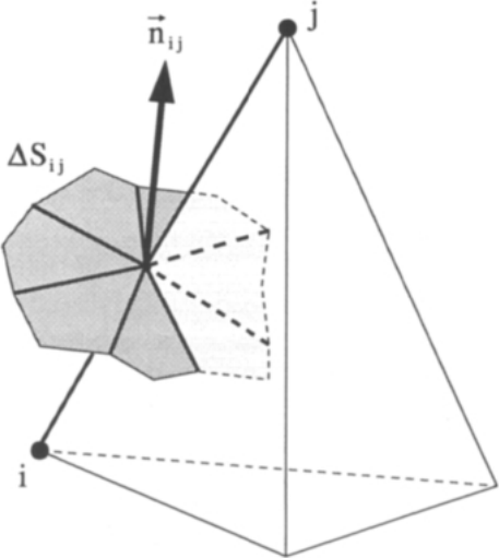
图5.9:三维中位对偶单元顶点格式中与边ij相关联的总面面积与平均单位法向量

图5.9:三维中位对偶单元顶点格式中与边 $$ij$$ 相关联的总面面积 $\Delta S_{ij}$ 与平均单位法向量 $\vec{n}_{ij}$ 。

通量的计算在形式上与单元中心格式所用的方法相同ï¼因此公式(5.18)-(5.22)在中位对偶格式中同样适用。如果采用上面这种把每条边与一个平均单位法向量相关联的做法ï¼那么最有效率的方法是在空间离散化中采用基于边(edge-based)的数据结构。这种数据结构对网格中每条具体的边(参见图5.9)存储:

指向定义该边的两个节点的指针——借此可以访问与两个控制体 $\Omega_i$ 和 $\Omega_j$ 相关联的流动变量;
面向量( $\vec{S}_{ij} = \vec{n}_{ij}\Delta S_{ij}$ )——必须一致地指向外侧或内侧;
从节点 $$i$$ 指向节点 $$j$$ 的边向量——把流动变量插值到面上(解的重构)时需要。另一种做法是ï¼边向量可以由节点坐标即时算得。对于带人工耗散的标准中心格式(5.3.1小节)ï¼此项并不需要。

The computation of fluxes follows formally the same approaches as for the cell-centred scheme. Thus, the formulae (5.18)-(5.22) are applicable also in the case of the median-dual scheme. If we utilise the above approach which associates each edge with a mean unit normal, the most efficient methodology is to employ an edge-based data structure for the spatial discretisation. The edge-based data structure stores for each particular edge in the grid (cf. Fig. 5.9):

pointers to the two nodes which define the edge - this allows us to access the flow variables associated with the two control volumes $\Omega_i$ and $\Omega_j$ ;
the face vector ( $\vec{S}_{ij} = \vec{n}_{ij}\Delta S_{ij}$ ) - must point consistently either outwards or inwards;
the edge vector from node $$i$$ to node $$j$$ - required for the interpolation of flow variables to the face (solution reconstruction). Alternatively, the edge vector can be computed on the fly from coordinates of the nodes. This is not required for the standard central scheme with artificial dissipation (Subsection 5.3.1).

这样ï¼通量的积分(例如按照方程(5.19))可以实现为对网格中所有边的一个循环:en

With this, the integration of the fluxes (e.g., according to Eq. (5.19)) would be implemented as a loop over all edges in the grid:

DO edge = 1, nedges
    i = pointer_to_left_node( edge )
    j = pointer_to_right_node( edge )
    (F dS)_ij = F(W_ij, n_ij) dS_ij   (approx.)
    R_i = R_i + (F dS)_ij
    R_j = R_j - (F dS)_ij
ENDDO

循环结束后ï¼再加上源项 $\vec{Q}_i\Omega_i$ ï¼就得到所有节点处的最终残差( $\vec{R}$ )。与对每个控制体分别累加通量相比ï¼这一方法的效率显著更高ï¼因为每个平均面向量只存储一次ï¼而且每条边也只访问一次而不是两次。此外ï¼由于我们使用完全相同的平均面向量 $\vec{S}_{ij}$ 来计算流入体积 $\Omega_i$ 和 $\Omega_j$ 的部分通量ï¼质量、动量和能量严格保持守恒。en

After the loop is completed and the source term $\vec{Q}_i\Omega_i$ is added, we obtain the final residuals ( $\vec{R}$ ) in all nodes. This approach is significantly more efficient than summing up the fluxes over each control volume separately, because we store each mean face vector only once and we also visit each edge only once instead of twice. Furthermore, since we use exactly the same mean face vector $\vec{S}_{ij}$ in order to to evaluate the partial fluxes into the volumes $\Omega_i$ and $\Omega_j$ , the mass, momentum and energy remain exactly conserved.