chapter. Boundary Conditions 第8章 边界条件[cfd-0009]
任何数值模拟都只能考虑真实物理域或系统的一部分。对求解域作截断会产生人工边界,在这些边界上我们必须给定某些物理量的值。此外,暴露于流动中的壁面构成物理域的自然边界。边界条件的数值处理需要格外细心:不当的实现会导致对真实系统的模拟不准确,此外求解格式的稳定性和收敛速度也会受到不利影响。en
Any numerical simulation can consider only a part of the real physical domain or of the system. The truncation of the domain leads to artificial boundaries, where we have to prescribe values of certain physical quantities. Furthermore, walls which are exposed to the flow represent natural boundaries of the physical domain. The numerical treatment of the boundary conditions requires a particular care. An improper implementation can result in an inaccurate simulation of the real system. Additionally, the stability and the convergence speed of the solution scheme can be negatively influenced.
在Euler方程与Navier-Stokes方程的数值求解中,通常会遇到下列几类边界条件:
- 固壁;
- 外流中的远场;
- 内流中的入流与出流;
- 喷注边界;
- 对称面;
- 坐标切割与周期边界;
- 网格块之间的边界。
en
The following types of boundary conditions are in general encountered in the numerical solution of the Euler and the Navier-Stokes equations:
- solid wall,
- farfield in external flows,
- inflow and outflow in internal flows,
- injection boundary,
- symmetry,
- coordinate cut and periodic boundary,
- boundary between blocks.
这些边界条件的数值处理将在下面几节中详细讨论。关于壁面热辐射、自由表面等其他边界条件的文献,读者可参阅3.4节。en
The numerical treatment of these boundary conditions is described in detail in the following sections. For literature on further boundary conditions like heat radiation on walls or like free surfaces, the reader is referred to Section 3.4.
8.1 Concept of Dummy Cells 虚单元的概念[cfd-8-1]
在继续讨论边界条件之前,我们应当提一下虚单元(dummy cells)或虚点(dummy points)的概念。这一做法在结构网格上非常流行,不过虚单元在非结构网格上也有一些优点。虚单元是物理域之外附加的网格单元层或点层。图8.1以二维结构网格为例对此作了示意。可以看到,整个计算域被两层虚单元(用虚线表示)包围。虚单元(点)通常不像域内网格那样生成(网格块之间的交界面除外):它们只是虚拟的单元,尽管体积、面向量等几何量也与之相关联。en
Before we proceed with the discussion of the boundary conditions, we should mention the concept of dummy cells or dummy points. This approach is very popular on structured grids. However, dummy cells offer some advantages also on unstructured grids. The dummy cells are additional layers of grid cells or points outside the physical domain. This is sketched in Fig. 8.1 for the case of a 2-D structured grid. As we can see, the whole computational domain is surrounded by two layers of dummy cells (denoted by dashed line). The dummy cells (points) are usually not generated as the grid inside the domain (except on interfaces between grid blocks). Rather, the cells are only virtual, although geometrical quantities like volumes or face vectors are associated with them.
虚单元的目的是简化边界上通量、梯度、耗散等的计算。其实现方式是把空间离散格式的模板(stencil)延伸到物理边界之外。如图8.1所示,在边界处可以采用与物理域内部相同的离散格式。这样,对所有“物理”网格点都能以同样的方式求解控制方程。这使离散格式易于实现。此外,结构网格的所有网格点可以在单个循环中遍历,这在向量计算机上具有显著优势。当然,前提是虚单元(点)中要存有守恒变量以及几何量的适当取值。显然,虚单元层的数目必须使模板位于物理域之外的部分被完全覆盖。虚单元(点)中的守恒变量由边界条件确定,几何量通常取自边界处相应的控制体。在多个网格块之间的边界情形(如图3.4),所有流动变量和几何量都从相邻块传递过来。en
The purpose of the dummy cells is to simplify the computation of the fluxes, gradients, dissipation, etc. along the boundaries. This is achieved by the possibility to extend the stencil of the spatial discretisation scheme beyond the physical boundaries. As we can see in Fig. 8.1, the same discretisation scheme can be employed at the boundaries as inside the physical domain. Thus, we can solve the governing equations in the same way for all "physical" grid points. This makes the discretisation schemes much easier to implement. Furthermore, all grid points of a structured grid can be accessed in a single loop, which is of significant advantage particularly on vector computers. The condition is of course that the dummy cells (points) contain appropriate values of the conservative variables as well as of the geometrical quantities. Clearly, the number of dummy cell layers must be such that the part of the stencil outside the physical domain is completely covered. The conservative variables in the dummy cells (points) are obtained from boundary conditions. The geometrical quantities are usually taken from the corresponding control volume at the boundary. In the case of boundaries between multiple grid blocks (like in Fig. 3.4), all flow variables and the geometry are transferred from the neighbouring block.
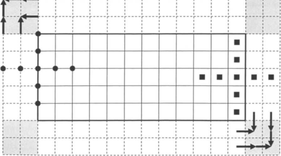
图8.1:二维计算域(粗线)周围的两层虚单元(虚线)。实心圆点表示二阶单元顶点(对偶)格式的标准模板,实心矩形勾画出二阶单元中心格式的模板(见4.3节)。
图8.1中灰色阴影的虚单元(及其相应点)带来一个难题:如果没有相邻的网格块,如何设置它们的取值并不十分明确。标准十字型离散模板并不需要它们的值。然而,这些单元(点)对梯度的计算(黏性通量——见4.4节)或多重网格中的转移算子(9.4节)十分重要。最简单的解决办法是由相邻的“规则”虚单元取平均,如图8.1中箭头所示。但这对于壁面或对称边界并不奏效。在这些情形下,更好的做法是把物理边界延伸到虚单元层中(参见CD-ROM上的结构化二维代码)。en
The grey-shaded dummy cells (and the associated points) in Fig. 8.1 represent a certain problem, since it is not quite clear how to set their values if there is no adjacent grid block. Their values are not required by the standard cross-type discretisation stencil. However, the cells (points) are important for the computation of gradients (viscous fluxes - see Section 4.4), or for the transfer operators within multigrid (Section 9.4). The simplest way to solve the problem is to average the values from the adjacent "regular" dummy cells, as indicated in Fig. 8.1 by arrows. However, this does not work satisfactorily for wall or symmetry boundaries. In these cases, it is better to extend the physical boundary into the dummy cell layers (see the structured 2-D code on the CD-ROM).
8.2 Solid Wall 固壁[cfd-8-2]
8.2.1 Inviscid Flow 无黏流动[cfd-8-2-1]
对于无黏流动,流体在表面上滑移。由于不存在摩擦力,速度矢量必定与表面相切。这等价于没有沿表面法向流动的条件,即en
In the case of an inviscid flow, the fluid slips over the surface. Since there is no friction force, the velocity vector must be tangent to the surface. This is equivalent to the condition that there is no flow normal to the surface, i.e.,
其中\(\vec{n}\)表示表面处的单位法向量。因此,逆变速度\(V\)(式(2.22))在壁面上为零。于是,对流通量向量式(2.21)只剩下压力项,即en
where \(\vec{n}\) denotes the unit normal vector at the surface. Hence, the contravariant velocity \(V\) (Eq. (2.22)) is zero at the wall. Consequently, the vector of convective fluxes Eq. (2.21) reduces to the pressure term alone, i.e,
其中\(p_w\)为壁面压力。en
with \(p_w\) being the wall pressure.
Structured Cell-Centred Scheme 结构化单元中心格式
在单元中心格式中,压力在单元的形心处求值。然而,式(8.2)中的\(p_w\)却需要取在边界单元的面上。最简便的做法是由域内外推得到壁面压力。参见图8.2,我们可以简单地取\(p_w=p_2\)。若采用两点公式en
Within the cell-centred scheme, the pressure is evaluated at the centroid of the cell. However, \(p_w\) in Eq. (8.2) is required at the face of the boundary cell. We can obtain the wall pressure most easily by extrapolation from the interior of the domain. Considering Fig. 8.2, we could simply set \(p_w=p_2\). Higher accuracy is achieved by using either a two-point
或三点外推公式en
or a three-point extrapolation formula
为了计及网格拉伸的影响,可以用到壁面的距离来代替其中的常数系数[1]。en
In order to account for grid stretching, distances to the wall could be employed instead of the constant coefficients [1].
上述外推公式(8.3)、(8.4)没有考虑网格与表面几何。另一种方法——所谓的法向动量关系(normal-momentum relation)——由Rizzi提出[2]。它基于这样一个事实:在无黏流动中壁面代表一条流线。把式(8.1)的法向零流动条件沿表面流线求导,并将结果代入动量方程,便得到en
The above extrapolation formulae (8.3), (8.4) do not account for the grid and the surface geometry. An alternative approach - the so-called normal-momentum relation - was developed by Rizzi [2]. It is based on the fact that the wall represents a streamline in inviscid flow. Differentiation of the zero-normal-flow condition in Eq. (8.1) along the surface streamline, and the substitution of the result into the momentum equation yields
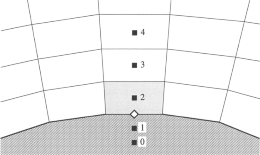
图8.2:单元中心格式的固壁边界条件。虚单元记为0和1。计算对流通量式(8.2)的位置用菱形标记。
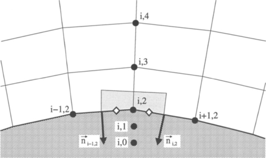
图8.3:结构化单元顶点对偶控制体格式的固壁边界条件。虚点记为(i,0)和(i,1)。计算对流通量式(8.2)的位置用菱形标出。另请对照图4.6中的示意。
式(8.5)把密度、速度和壁面几何与压力的法向导数联系起来。已经证明,法向动量关系能给出非常精确的结果[1]。然而,在复杂几何情形下,法向动量关系的数值求解可能出现问题。实现的详细描述与精度比较见文献[1]。en
Equation (8.5) relates the density, the velocity and the wall geometry to the normal derivative of the pressure. It was demonstrated that the normal-momentum relation gives very accurate results [1]. However, problems can arise with the numerical solution of the normal-momentum relation in the case of complex geometries. Detailed description of the implementation and accuracy comparisons can be found in Ref. [1].
虚单元中守恒变量的取值可以由域内线性外推得到,即en
The values of the conservative variables in the dummy cells can be obtained by linear extrapolation from the interior, i.e.,
Structured Cell-Vertex Scheme 结构化单元顶点格式
对于具有重叠控制体的单元顶点离散格式(小节4.2.2),边界条件式(8.1)的实现很直接。壁面上的对流通量按式(8.2)计算。壁面压力\(p_w\)通过节点值平均得到:二维情形如式(4.26)所示,三维情形如式(4.27)所示。分布公式(二维为式(4.30))此时只涉及两个(三维为四个)单元(请比较图4.4与图8.3)。en
The implementation of the boundary condition Eq. (8.1) is straightforward for the cell-vertex discretisation scheme with overlapping control volumes (Subsection 4.2.2). The convective fluxes at the wall faces are computed according to Eq. (8.2). The wall pressure \(p_w\) is obtained by averaging the nodal values as indicated in Eq. (4.26) for a 2-D, or in Eq. (4.27) for a 3-D case. The distribution formula (Eq. (4.30) in 2D) accounts now for only two (four in 3D) cells (compare Fig. 4.4 to Fig. 8.3).
对于具有对偶控制体的单元顶点格式(小节4.2.3),可以采用几种不同的做法。一种做法是对位于壁面上的控制体的每个面分别应用式(8.2)中的条件。于是,按照图8.3,可以写出en
Several different ways can be followed in the case of the cell-vertex scheme with dual control volumes (Subsection 4.2.3). One approach is to apply the condition in Eq. (8.2) separately for each face of the control volume which is on the wall. Thus, according to Fig. 8.3, we can write
相应的三维公式将在后面非结构网格小节中给出。en
The corresponding 3-D formula will be presented further below in the subsection on unstructured grids.
另一种可行做法是直接在相应壁面节点处(即图8.3中的节点\((i,2)\))应用式(8.2)中的条件。壁面压力\(p_w\)直接取为\(p_{i,2}\)。单位法向量取为共享节点\((i,2)\)的所有壁面小面(facet)法向量的平均。这一做法需要对速度矢量作修正:在用时间推进格式更新解之后,把壁面上的速度矢量投影到切平面上[3]、[4],即en
Another possible implementation employs the condition in Eq. (8.2) directly in the respective wall node (i.e., node \((i,2)\) in Fig. 8.3). The wall pressure \(p_w\) is simply set equal to \(p_{i,2}\). The unit normal vector is computed as the average of the normal vectors of all wall facets which share the node \((i,2)\). This approach requires a correction of the velocity vector. After the solution update by the time-stepping scheme, the velocity vector at the wall is projected onto the tangential plane [3], [4], i.e.,
其中\(\vec{n}_{av}\)为平均后的单位法向量。这样,流动将与壁面相切。en
with \(\vec{n}_{av}\) being the averaged unit normal vector. In this way, the flow will become tangential to the wall.
Unstructured Cell-Centred Scheme 非结构单元中心格式
式(8.1)的壁面边界条件在非结构单元中心格式中的实现方式与结构网格类似。如果边界单元是四边形、六面体或棱柱(壁面为三角形的面),可以用式(8.3)把压力外推到壁面。相邻单元(图8.2中的3号单元)可由小节5.2.1所述的基于面的数据结构得到。对于三角形或四面体单元,文献[5]和[6]建议采用一层虚单元,虚单元中的速度分量通过把边界单元的速度矢量关于壁面反射得到。例如,在图8.2中的虚单元1内,速度变为en
The wall boundary condition in Eq. (8.1) can be implemented for a cell-centred unstructured scheme in a way similar to that on structured grids. If the boundary cell is a quadrilateral, hexahedron or a prism (with triangular face on the wall), the pressure can be extrapolated to the wall by using Eq. (8.3). The neighbouring cell (number 3 in Fig. 8.2) is known from the face-based data structure described in Subsection 5.2.1. For the case of a triangular or tetrahedral cell, in Ref. [5] and [6] it was suggested to employ one layer of dummy cells. The velocity components in the dummy cells were obtained by reflecting the velocity vectors in the boundary cells at the wall. For example, in the dummy cell 1 in Fig. 8.2, the velocity would become
其中\(V_2=u_2n_x+v_2n_y+w_2n_z\)为逆变速度,\(\vec{n}=[n_x,n_y,n_z]^T\)表示壁面单位法向量。虚单元中的压力和密度取为与相应边界单元中的值相等(这意味着\(p_w=p_2\))。en
where \(V_2=u_2n_x+v_2n_y+w_2n_z\) is the contravariant velocity and \(\vec{n}=[n_x,n_y,n_z]^T\) stands for the wall unit-normal vector. The pressure and density in the dummy cells were set equal to the values in the corresponding boundary cell (this implies \(p_w=p_2\)).
Unstructured Median-Dual Scheme 非结构中位对偶格式
在非结构中位对偶(median-dual)离散格式的情形下,边界条件式(8.1)需要更多的注意。二维情形如图8.4所示,三维情形如图8.5所示。式(8.2)的对流通量在位于壁面上的控制体每个面处分别计算。这与上文针对具有对偶控制体的结构化单元顶点格式讨论的第一种做法相同。对于四边形元素(如图8.4中的1-3-4-5),压力按与式(8.8)相应的方式插值。对于六面体、棱柱或棱锥,其控制体面为四边形(如图8.5中的面1-4-5-6),插值公式为en
The boundary condition Eq. (8.1) requires more attention in the case of the median-dual unstructured discretisation scheme. The situation is shown in Fig. 8.4 for the 2-D and in Fig. 8.5 for the 3-D case. The convective fluxes in Eq. (8.2) are computed separately at each face of the control volume which is located on the wall. This is identical to the first approach discussed above for the structured cell-vertex scheme with dual control volumes. For quadrilateral elements (like 1-3-4-5 in Fig. 8.4), the pressure is interpolated correspondingly to Eq. (8.8). In the case of hexahedra, prisms or pyramids, where the face of the control volume is a quadrilateral (like face 1-4-5-6 in Fig. 8.5), the interpolation formula reads
如果边界元素是四面体或棱柱(二维情形为三角形),壁面上的压力应当按有限元方法计算en
If the boundary elements are tetrahedra or prisms (or triangles in 2-D), the pressure at the wall face should be evaluated like in the finite element method
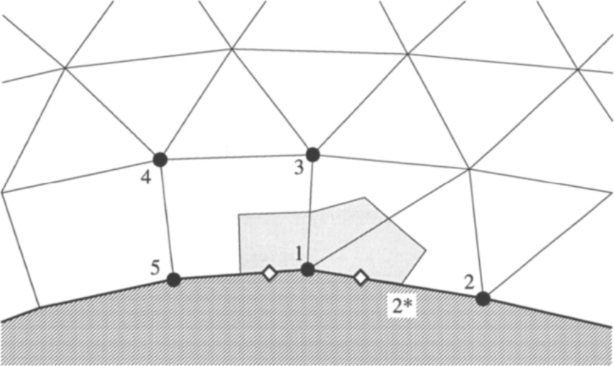
图8.4:二维非结构对偶控制体混合网格格式的固壁边界条件。计算对流通量式(8.2)的位置用菱形标出。
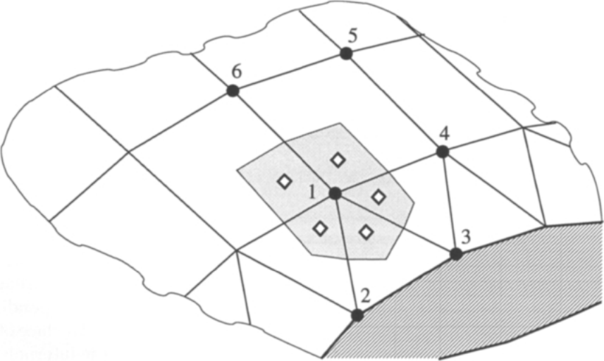
图8.5:三维非结构混合网格格式的固壁边界条件。计算对流通量式(8.2)的位置用菱形标出。
[7]。例如,对于图8.4中的壁面段1-2,面1-2*上的压力应按下式计算en
[7]. At the wall segment 1-2 in Fig. 8.4 for example, the pressure at the face 1-2* would be computed as
对于四面体,例如图8.5中的壁面1-2-3,压力按下式计算en
In the case of a tetrahedra with, e.g., the wall face 1-2-3 in Fig. 8.5, the pressure is evaluated as
应当强调,这种有限元型插值对获得准确的流动解十分重要[7]。en
It should be stressed that this finite-element type interpolation is important for an accurate flow solution [7].
8.2.2 Viscous Flow 黏性流动[cfd-8-2-2]
对于流经固壁的黏性流体,假设表面与紧贴表面的流体之间的相对速度为零。因此,我们称之为无滑移(noslip)边界条件。对于固定的壁面,笛卡儿速度分量变为en
For a viscous fluid which passes a solid wall, the relative velocity between the surface and the fluid directly at the surface is assumed to be zero. Therefore, we speak of noslip boundary condition. In the case of a stationary wall surface, the Cartesian velocity components become
无滑移条件带来两个基本推论。第一,我们不需要在壁面上求解动量方程——单元顶点格式正是利用了这一点。第二,通过无滑移壁面的对流通量仍由式(8.2)给出,而式(2.24)中的各项简化为\(\vec{\Theta}=k\vec{\nabla}T\)。因此,对流通量中的壁面压力仍按上文无黏流动中所述的方式求得。不过,虚单元(点)的处理方式有所不同。en
There are two basic consequences of the noslip condition. First, we do not need to solve the momentum equations on the wall. This fact is utilised in the cell-vertex scheme. Second, the convective fluxes through the noslip wall are given again by Eq. (8.2), and the terms in Eq. (2.24) simplify to \(\vec{\Theta}=k\vec{\nabla}T\). Hence, the wall pressure in the convective fluxes is obtained in the same way as described above for the inviscid flow. However, the dummy cells (points) are treated in a different way.
Cell-Centred Scheme 单元中心格式
对单元0和3同理。这一做法既适用于结构格式,也适用于非结构格式(参见文献[6])。en
and likewise for the cells 0 and 3. The approach is applicable to both, structured and unstructured schemes (cf. Ref. [6]).
如果给定壁温,速度分量仍按式(8.15)那样反号。虚单元中的温度利用给定的壁温从内场线性外推。由于垂直于壁面的压力梯度为零,边界元素中的压力也规定用于虚单元(即\(p_0=p_1=p_2\))。虚单元中的密度和总能由插值得到的值算出。en
If the wall temperature is given, the velocity components are still reversed as in Eq. (8.15). The temperature in the dummy cells is linearly extrapolated from the interior field by using the specified wall temperature. Since the pressure gradient normal to the wall is zero, the pressure in the boundary element is prescribed also in the dummy cells (i.e., \(p_0=p_1=p_2\)). The density and the total energy in the dummy cells are evaluated from the interpolated values.
Cell-Vertex Scheme 单元顶点格式
由于不必求解动量方程,壁面上没有来自对流通量(式(8.2))的贡献。式(2.23)的黏性通量对能量方程只贡献垂直于壁面的温度梯度。对于绝热壁,\(\vec{\nabla}T_w\cdot\vec{n}\)为零。因此,我们完全不必计算通过壁面的对流通量或黏性通量。为了防止在壁面节点上产生非零速度分量,应把动量方程的残差置零。en
Since the momentum equations need not to be solved, there is no contribution from the convective fluxes (Eq. (8.2)) at the wall. The viscous fluxes in Eq. (2.23) contribute only the temperature gradient normal to the wall to the energy equation. For an adiabatic wall, \(\vec{\nabla}T_w\cdot\vec{n}\) is zero. Hence, we do not have to compute any convective or viscous fluxes through the wall. The residuals of the momentum equations should be set to zero, in order to prevent the generation of nonzero velocity components at the wall nodes.
如果给定壁温,在完全气体假设下可以直接设置壁面上的总能(例如图8.3中的节点\((i,2)\))en
In the case of a prescribed wall temperature, we can directly set the total energy at the wall (e.g., node \((i,2)\) in Fig. 8.3) using (perfect gas assumed)
其中\(T_w\)表示给定的壁温。动量方程和能量方程的残差都必须置零。同一策略也适用于非结构格式。en
where \(T_w\) denotes the given wall temperature. The residuals of the momentum and of the energy equation have to be zeroed out. The same strategy is applicable also to unstructured schemes.
对于非绝热壁,另一种做法在某些应用中似乎更为稳健:它完全不在壁面上求解控制方程,而是直接给定密度和能量en
Another approach for non-adiabatic walls, which seems to be more robust for some applications, does not solve the governing equations at the wall at all. Both, the density and the energy are directly specified
式(8.17)中的关系假设垂直于壁面没有压力梯度(因此\(p_{i,2}=p_{i,3}\))。由于所有守恒变量都已给定,\((i,2)\)处所有方程的残差都应置零。该技术同样可用于非结构网格。不过,在三角形或四面体网格上,压力的外推需要额外的运算。en
The relations in Eq. (8.17) assume that there is no pressure gradient normal to the wall (therefore \(p_{i,2}=p_{i,3}\)). Since all conservative variables are prescribed, the residuals of all equations should be set to zero at \((i,2)\). This technique can be utilised on unstructured grids as well. However, the extrapolation of the pressure requires additional operations on triangular or tetrahedral grids.
如果壁面绝热,虚点中的值按如下方式得到en
If the wall is adiabatic, the values in the dummy points are obtained as follows
对节点0和4同样如此。如果给定壁温,虚点中的温度由内场外推,即en
The same applies to the nodes 0 and 4. If the wall temperature is given, the temperature in the dummy points is extrapolated from the interior, i.e.,
8.3 Farfield 远场[cfd-8-3]
绕翼型、机翼、汽车及其他外形的外流数值模拟必须在有界域内进行,因此人工远场边界条件成为必需。远场边界条件的数值实现须满足两个基本要求:第一,与无限域相比,求解域的截断不应对流动解产生明显影响;第二,任何向外传播的扰动都不得被反射回流场[9]。由于其椭圆性质,亚声速与跨声速流动问题对远场边界条件特别敏感。不当的实现会显著减慢向定常态的收敛,而且解的精度也很可能受到不利影响。人们已发展出多种能够在人工边界处吸收外传波的方法[10]-[15]。关于各种无反射边界条件的综述可见[16]。en
The numerical simulation of external flows past airfoils, wings, cars and other configurations has to be conducted within a bounded domain. For this reason, artificial farfield boundary conditions become necessary. The numerical implementation of the farfield boundary conditions has to fulfil two basic requirements. First, the truncation of the domain should have no notable effects on the flow solution as compared to the infinite domain. Second, any outgoing disturbances must not be reflected back into the flow field [9]. Due to their elliptic nature, sub- and transonic flow problems are particularly sensitive to the farfield boundary conditions. An inadequate implementation can lead to a significant slow down of convergence to the steady state. Furthermore, the accuracy of the solution is likely to be negatively influenced. Various methodologies were developed, which are capable of absorbing the outgoing waves at the artificial boundaries [10]-[15]. An review of different non-reflecting boundary conditions can be found in [16].
在下面两个小节中,我们将讨论Whitfield和Janus[12]所述的特征变量(characteristic variables)概念,并给出针对升力体的远场边界条件扩展。en
In the following two subsections, we shall discuss the concept of characteristic variables as it was described by Whitfield and Janus [12]. We shall also present an extension of the farfield boundary conditions for lifting bodies.
8.3.1 Concept of Characteristic Variables 特征变量的概念[cfd-8-3-1]
信息沿特征线流出或流入计算域,取决于对流通量雅可比矩阵特征值的符号(附录A.11,式(A.84)或(A.88))。例如,亚声速入流时有四条入射特征线(三维)和一条出射特征线(式(A.88)中的\(\lambda_5\));亚声速出流时情形正好相反。根据Kreiss的一维理论[17],在边界上从域外施加的条件数应等于入射特征线的条数,其余条件应由域内的解确定。en
Depending on the sign of the eigenvalues of the convective flux Jacobians (Appendix A.11, Eq. (A.84) or (A.88)), the information is transported out of or into the computational domain along the characteristics. For example, in the case of subsonic inflow there are four incoming characteristics (in 3D) and one outgoing (\(\lambda_5\) in Eq. (A.88)). The situation reverses for subsonic outflow. According to the one-dimensional theory of Kreiss [17], the number of conditions to be imposed from outside at the boundary should be equal to the number of incoming characteristics. The remaining conditions should be determined from the solution inside the domain.
Whitfield和Janus的方法[12]基于边界法向方向上Euler方程(2.45)的特征形式。实践表明,该方法在结构与非结构网格上对多种流动情形都表现很好。它不仅可用于远场边界,也可用于无黏固壁(小节8.2.1)。en
The approach of Whitfield and Janus [12] is based on the characteristic form of the Euler equations (2.45) normal to the boundary. The methodology was found to perform very well on structured and unstructured grids in a large variety of flow cases. It can be applied not only to farfield boundaries but also to inviscid solid walls (Subsection 8.2.1).
远场边界处的两种基本流动情形绘于图8.6。流动既可能进入也可能离开计算域。因此,依局部马赫数不同,需要处理四种不同类型的远场边界条件:
- 超声速入流;
- 超声速出流;
- 亚声速入流;
- 亚声速出流。
en
The two basic flow situations at the farfield boundary are sketched in Fig. 8.6. The flow can either enter or it can leave the domain. Therefore, depending on the local Mach number, four different types of farfield boundary conditions have to be treated:
- supersonic inflow,
- supersonic outflow,
- subsonic inflow, and
- subsonic outflow.
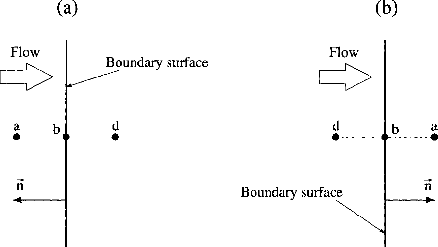
图8.6:远场边界:入流(a)与出流(b)情形。位置\(a\)在域外,\(b\)在边界上,位置\(d\)在物理域内。单位法向量\(\vec{n}=[n_x,n_y,n_z]^T\)指向域外。图例:Flow——流动;Boundary surface——边界面。
Supersonic Inflow 超声速入流
对于超声速入流,所有特征值同号。由于流动进入物理域,边界上(图8.6中的点\(b\))的守恒变量完全由自由来流值确定,即en
For supersonic inflow, all eigenvalues have the same sign. Since the flow is entering the physical domain, the conservative variables on the boundary (point \(b\) in Fig. 8.6) are determined by freestream values only. Thus,
\(\vec{W}_a\)的值根据给定的马赫数\(M_\infty\)和两个气流角(迎角、侧滑角)确定。en
The values \(\vec{W}_a\) are specified based on the given Mach number \(M_\infty\) and on two flow angles (angle of attack, side-slip angle).
Supersonic Outflow 超声速出流
这种情形下所有特征值同样同号。但此时流动离开物理域,边界上所有守恒变量都必须由域内的解确定,只需令en
In this case, all eigenvalues have also the same sign. However, the flow leaves now the physical domain and all conservative variables at the boundary must be determined from the solution inside the domain. This can be accomplished simply by setting
Subsonic Inflow 亚声速入流
此时,四条特征线进入、一条离开物理域。因此,四个特征变量根据自由来流值给定,一个特征变量由物理域内外推。由此得到下列边界条件[12]en
Here, four characteristics enter and one leaves the physical domain. Therefore, four characteristic variables are prescribed based on the freestream values. One characteristic variable is extrapolated from the interior of the physical domain. This leads to the following set of boundary conditions [12]
其中\(\rho_0\)和\(c_0\)表示一个参考状态。参考状态通常取为内点处(图8.6中的点\(d\))的状态。点\(a\)处的值由自由来流状态确定。en
where \(\rho_0\) and \(c_0\) represent a reference state. The reference state is normally set equal to the state at the interior point (point \(d\) in Fig. 8.6). The values in point \(a\) are determined from the freestream state.
Subsonic Outflow 亚声速出流
对于亚声速出流,四个流动变量(密度和三个速度分量)必须由物理域内部外推得到,余下的第五个变量(压力)必须从外部给定。远场边界处的原始变量由下式得到[12]en
In the case of subsonic outflow, four flow variables (density and the three velocity components) have to be extrapolated from the interior of the physical domain. The remaining fifth variable (pressure) must be specified externally. The primitive variables at the farfield boundary are obtained from [12]
其中\(p_a\)为给定的静压。en
with \(p_a\) being the prescribed static pressure.
虚单元中的物理量可由状态\(b\)和\(d\)线性外推得到。en
Physical properties in the dummy cells can be obtained by linear extrapolation from the states \(b\) and \(d\).
8.3.2 Modifications for Lifting Bodies 升力体情形的修正[cfd-8-3-2]
上述特征远场边界条件假设环量为零,这对亚声速或跨声速流动中的升力体并不正确。因此,远场边界必须放在离物体非常远的地方,否则流动解会不准确。如果自由来流中包含一个单独涡的影响(三维情形为马蹄涡),到远场的距离可以显著缩短(约一个数量级)。该涡假定位于升力体的中心,其强度与物体产生的升力成正比。下面我们给出涡修正的二维和三维实现。en
The above characteristic farfield boundary conditions assume zero circulation, which is not correct for a lifting body in sub- or transonic flow. For this reason, the farfield boundary has to be located very far away from the body. Otherwise, the flow solution will be inaccurate. The distance to the farfield can be significantly shortened (by one order of magnitude), if the freestream flow includes the effect of a single vortex (horse-shoe vortex in 3D). The vortex is assumed to be centred at the lifting body. The strength of the vortex is proportional to the lift produced by the body. In the following, we shall present implementations of the vortex correction in 2D and in 3D.
Vortex Correction in 2D 二维涡修正
这里要叙述的方法由Usab和Murman提出[18]。修正后自由来流速度的分量由下列表达式给出(假设可压缩流动)en
The approach, which we want to describe here, was suggested by Usab and Murman [18]. The components of the corrected freestream velocity are given by the expressions (compressible flow assumed)
其中\(\Gamma\)为环量,\((d,\theta)\)为远场点的极坐标,\(\alpha\)为迎角,\(M_\infty\)为自由来流马赫数。环量由下式求得en
with \(\Gamma\) being the circulation, \((d,\theta)\) the polar coordinates of the farfield point, \(\alpha\) the angle of attack, and \(M_\infty\) denoting the freestream Mach number, respectively. The circulation is obtained from
其中\(x_{ref}\)和\(y_{ref}\)为参考点(涡所在位置,例如1/4弦长处)的坐标。en
where \(x_{ref}\) and \(y_{ref}\) are the coordinates of the reference point (location of the vortex - e.g., at 1/4 chord).
修正后的自由来流压力\(p_\infty^{*}\)由下式给出en
The modified freestream pressure \(p_\infty^{*}\) is given by
其中\(\|\vec{v}_\infty^{*}\|_2^2=(u_\infty^{*})^2+(v_\infty^{*})^2\)。修正后的自由来流密度由状态方程得到en
with \(\|\vec{v}_\infty^{*}\|_2^2=(u_\infty^{*})^2+(v_\infty^{*})^2\). The corrected freestream density is obtained from the equation of the state
上述涡修正式(8.24)-(8.28)严格来说只对亚声速流动成立。不过,实践证明对自由来流条件的这一修正在跨声速流动中同样有帮助。图8.7展示了这方面的结果,其中研究了升力系数对远场边界距离的依赖关系。远场半径取为5、20、50和99倍弦长。可以看到,不加涡修正的模拟对远场距离有强烈的依赖性;相反,带涡的模拟在约20倍弦长的距离内仍保持足够精度。这使网格单元/点数显著减少。文献[19]证明,若在涡修正中使用更高阶的项,远场边界可以只放在约5倍弦长处而不损失精度。en
The above vortex correction Eqs. (8.24)-(8.28) is strictly valid for subsonic flow only. However, the modification of the freestream conditions proved to be helpful in transonic flow as well. This is demonstrated in Fig. 8.7, where the dependence of the lift coefficient on the distance to the farfield boundary was investigated. The farfield radius was set to 5, 20, 50, and 99 chords. As we can see, simulations without the vortex correction experiences a strong dependence on the farfield distance. On the contrary, simulations with the vortex remain sufficiently accurate up to a distance of about 20 chords. This leads to a significant reduction of the number of grid cells/points. It was demonstrated in Ref. [19] that by using higher-order terms in the vortex correction, the farfield boundary can be placed only about 5 chords away without loss of accuracy.
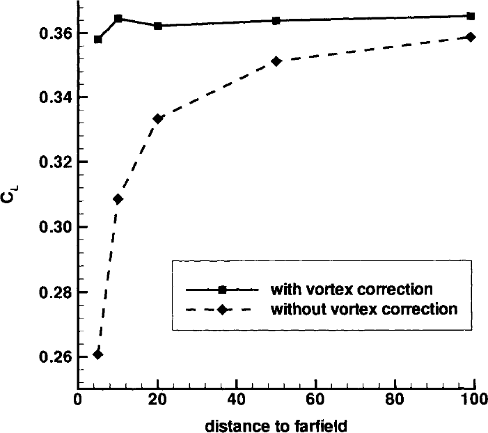
图8.7:到远场边界的距离和单个涡对升力系数的影响。NACA 0012翼型,\(M_\infty=0.8\),\(\alpha=1.25^{\circ}\)。图例:横轴distance to farfield——到远场的距离;纵轴\(C_L\)——升力系数;with vortex correction——带涡修正;without vortex correction——不带涡修正。
Vortex Correction in 3D 三维涡修正
机翼对远场边界的影响可以用马蹄涡来近似。对于可压缩流动,修正后的自由来流速度分量可由下式得到[20]、[21]en
The effect of a wing on the farfield boundary can be approximated by a horse-shoe vortex. In the case of compressible flow, the modified freestream velocity components can be obtained from [20], [21]
其中\(\Gamma\)表示环量,\((x,y,z)\)为远场点的笛卡儿坐标,\(l\)为半展长。此外,式(8.29)中假设流动沿正\(x\)方向,机翼沿\(z\)轴布置。式(8.29)中的\(\mathcal{A}\)、\(\mathcal{B}\)和\(\mathcal{C}\)为en
where \(\Gamma\) denotes the circulation, \((x,y,z)\) the Cartesian coordinates of the farfield point, and \(l\) stands for the half span, respectively. Furthermore, in Eq. (8.29) it was assumed that the flow is in the positive \(x\)-direction with the wing being oriented along the \(z\)-axis. The terms \(\mathcal{A}\), \(\mathcal{B}\) and \(\mathcal{C}\) in Eq. (8.29) read
其中缩写定义为en
The abbreviations are given by
其中\(M_\infty\)为自由来流马赫数。环量\(\Gamma\)仍用式(8.25)计算,此时\(a\)表示平均弦长。修正后的压力(\(p_\infty^{*}\))和密度(\(\rho_\infty^{*}\))分别由公式(8.27)和(8.28)求得。式(8.22)或式(8.23)中的\(u_a\)、\(v_a\)、\(w_a\)、\(p_a\)和\(\rho_a\)替换为其修正值\(u_\infty^{*}\)、\(v_\infty^{*}\)、\(w_\infty^{*}\)、\(p_\infty^{*}\)和\(\rho_\infty^{*}\)。en
with \(M_\infty\) being the freestream Mach number. The circulation \(\Gamma\) is calculated using Eq. (8.25), where \(a\) represents the mean chord. The corrected values of pressure (\(p_\infty^{*}\)) and of density (\(\rho_\infty^{*}\)) are obtained from the formulae (8.27) and (8.28), respectively. The quantities \(u_a\), \(v_a\), \(w_a\), \(p_a\), and \(\rho_a\) in Eq. (8.22) or Eq. (8.23) are replaced by their corrected values \(u_\infty^{*}\), \(v_\infty^{*}\), \(w_\infty^{*}\), \(p_\infty^{*}\), and \(\rho_\infty^{*}\).
以及\(x=x_{farf}\)。为避免数值奇性,文献[21]建议把en
and \(x=x_{farf}\). In order to avoid the numerical singularity, in Ref. [21] it was suggested to constrain the values of
在式(8.29)中的取值限制在1/4展长,即\(l/2\)以内。这一措施把涡线\(z=l\)和\(z=-l\)周围\(l/2\)距离内对速度\(v_\infty\)和\(w_\infty\)的修正量减小。en
in Eq. (8.29) to the 1/4 wingspan, i.e., \(l/2\). This measure reduces the corrections to the velocities \(v_\infty\) and \(w_\infty\) within the distance \(l/2\) around the vortex lines \(z=l\) and \(z=-l\).
文献[21]给出的数值结果表明,应用式(8.29)的涡修正后,升力系数和阻力系数对远场距离的敏感性降低。研究发现,到远场边界\(7\cdot l\)的距离足以获得准确的结果。en
The numerical results presented in [21] indicate a reduced sensitivity of the lift and drag coefficient with respect to the farfield distance, if the vortex correction in Eq. (8.29) is applied. It was found that a distance of \(7\cdot l\) to the farfield boundary is sufficient for accurate results.
8.4 Inlet/Outlet Boundary 入流/出流边界[cfd-8-4]
针对Navier-Stokes方程的数值入流、特别是出流(也称为开放,open)边界条件的实现,已提出了多种方法[22]-[26]。这里我们集中讨论为叶轮机械应用而发展的方法。合适的无反射入流与出流边界条件可参见例如[27]-[30]。Giles[31]以及Hirsch和Verhoff[32]为Euler方程提出了无反射边界条件,适用于物体与入流或出流平面之间距离较短的求解域。en
Various approaches were devised for the implementation of numerical inlet, and in particular, of outlet (also named open) boundary conditions for the Navier-Stokes equations [22]-[26]. Here, we will concentrate on methodologies, which were developed for turbomachinery applications. Suitable non-reflecting inlet and outlet boundary conditions were described, e.g., in [27]-[30]. Giles [31], and Hirsch and Verhoff [32] suggested non-reflecting boundary conditions for the Euler equations, which are intended for domains with a short distance between the body and the inlet or the outlet plane.
在某些情形下,入流和出流边界除速度外,其压力梯度和温度梯度也是周期性的。例如在换热器的模拟中就会遇到这类流动[33]。针对槽道LES的周期入流和出流边界条件的实现见[34]-[36]。en
In certain cases, the inlet and outlet boundary are additionally periodic with respect to the velocity as well as the pressure and temperature gradient. This type of flow is encountered, for example, in the simulation of heat exchangers [33]. The implementation of periodic inlet and outlet boundary conditions was presented in [34]-[36] for LES in channels.
Subsonic Inlet 亚声速入流
常用的做法是给定总压、总温和两个气流角。有一个特征变量需要从流动域内插值。一种可能的做法是利用外传黎曼不变量(Riemann invariant)[30],其定义为en
A common procedure consists of the specification of the total pressure, total temperature, and of two flow angles. One characteristic variable has to be interpolated from the interior of the flow domain. One possibility is to employ the outgoing Riemann invariant [30], which is defined as
其中下标\(d\)表示域内状态(参见图8.6a)。黎曼不变量用来确定边界上的绝对速度或声速。实践中发现,选取声速会得到更稳定的格式,对低马赫数流动尤其如此。因此,我们令en
where the index \(d\) denotes the state inside the domain (cf. Fig. 8.6a). The Riemann invariant is used to determine either the absolute velocity or the the speed of sound at the boundary. In practice, it was found that selecting the speed of sound leads to a more stable scheme, particularly for low Mach-number flows. Therefore, we set
其中\(\theta\)为相对于边界的气流角,\(c_0\)表示滞止声速。于是en
with \(\theta\) being the flow angle relative to the boundary, and \(c_0\) denoting the stagnation speed of sound. Hence,
以及en
and
边界上的静温、静压、密度或绝对速度等量按如下方式求值en
Quantities like the static temperature, pressure, density, or the absolute velocity at the boundary are evaluated as follows
其中\(T_0\)和\(p_0\)为给定的总温和总压,\(R\)和\(c_p\)分别表示气体常数和定压比热。入口处的速度分量通过按两个(二维为一个)给定的气流角分解\(\|\vec{v}_b\|_2\)得到。en
where \(T_0\) and \(p_0\) are the given values of total temperature and pressure, \(R\) and \(c_p\) represent the specific gas constant and the heat coefficient at constant pressure, respectively. The velocity components at the inlet are obtained by decomposing \(\|\vec{v}_b\|_2\) according to the two (one in 2D) prescribed flow angles.
Subsonic Outlet 亚声速出流
在叶轮机械中,出口处通常给定静压。亚声速出流边界的处理方式与式(8.23)的出流条件非常相似,只是把环境压力\(p_a\)换成给定的出口静压。en
In turbomachinery, the static pressure is usually prescribed at the outlet. The subsonic outlet boundary can be treated in a way quite similar to the outflow condition in Eq. (8.23). Only the ambient pressure \(p_a\) is replaced here by the given static exit pressure.
虚单元(点)中的流动变量可以通过对边界处和内点\(d\)处的状态作线性外推得到。en
Flow variables in the dummy cells (points) can be obtained by linearly extrapolating the states at the boundary and at the interior point \(d\).
8.5 Injection Boundary 注入边界[cfd-8-5]
注入速度和其他流动变量由给定的质量流量\(\dot{m}\)与注入温度\(T_{inj}\)算出。这里我们假设质量流沿垂直于边界的方向注入。对流通量用式(2.21)计算,并把逆变速度\(V\)取为注入速度,即en
The injection velocity and other flow variables are computed from the given mass flow rate \(\dot{m}\) and the injection temperature \(T_{inj}\). We will assume here that the mass is injected perpendicular to the boundary. The convective fluxes are evaluated using Eq. (2.21) with the contravariant velocity \(V\) set equal to the injection velocity, i.e.,
速度分量利用面法向量按下式求值en
Velocity components are evaluated using the face normal vector as
对于图8.8a中所描绘的单元中心格式,\(p_b\)可以直接取为边界单元内的压力,即\(p_b=p_2\)。中位对偶单元顶点格式则需要由定义相应面面积的各点插值\(p_b\)(即由图8.8b中的\((i,2)\)和\((i+1,2)\)插值)。为此可以利用式(8.8)、(8.11)-(8.13)之类的公式。虚单元(点)中的值由域内作零阶外推或线性外推得到。en
For the cell-centred scheme sketched in Fig. 8.8a, \(p_b\) can be set identical to the pressure in the boundary cell, i.e., \(p_b=p_2\). The median-dual cell-vertex scheme requires an interpolation of \(p_b\) from the points defining the particular face area (i.e., from \((i,2)\) and \((i+1,2)\) in Fig. 8.8b). Formulae like (8.8), (8.11)-(8.13) can be utilised for this purpose. Values in the dummy cells (points) are obtained by 0-th order or by linear extrapolation from the interior.
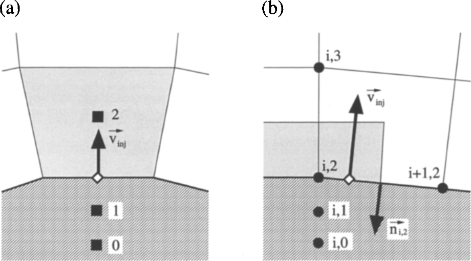
图8.8:结构化单元中心格式(a)与单元顶点对偶控制体格式(b)的注入边界条件。虚单元(点)记为1和0。计算对流通量的位置用菱形标出。
8.6 Symmetry Plane 对称面[cfd-8-6]
如果流动相对于某条直线或某个平面是对称的,那么首先必须满足的条件是边界上没有通量通过。这等价于要求垂直于对称边界的速度为零。此外,下列梯度必须为零:
- 标量在垂直于边界方向上的梯度;
- 切向速度在垂直于边界方向上的梯度;
- 法向速度沿边界方向的梯度(因为\(\vec{v}\cdot\vec{n}=0\))。
en
If the flow is to be symmetrical with respect to a line or a plane, the first condition which must be met is that there is no flux across the boundary. This is equivalent to the requirement that the velocity normal to the symmetry boundary is zero. Furthermore, the following gradients have to vanish:
- gradient of a scalar quantity normal to the boundary,
- gradient of the tangential velocity normal to the boundary,
- gradient of the normal velocity along the boundary (since \(\vec{v}\cdot\vec{n}=0\)).
这些条件可以写为en
We can write these conditions as
其中\(U\)表示标量变量,\(\vec{t}\)表示与对称边界相切的向量。en
where \(U\) stands for a scalar variable and \(\vec{t}\) denotes a vector tangential to the symmetry boundary.
Cell-Centred Scheme 单元中心格式
采用虚单元可以大大简化对称边界条件的实现。虚单元中的流动变量利用镜像单元(reflected cells)的概念得到。也就是说,虚单元中密度、压力等标量取为对面内部单元中的值,即en
The implementation of the symmetry boundary condition can be largely simplified by employing dummy cells. The flow variables in the dummy cells are obtained using the concept of reflected cells. This means that scalar quantities like density or pressure in the dummy cells are set equal to the values in the opposite interior cells, i.e.,
记号与图8.2一致。速度分量按式(8.10)所示相对于边界作反射。虚单元中法向速度的法向梯度与对面内部单元中的相等,但符号相反。en
The notation corresponds to that in Fig. 8.2. The velocity components are reflected with respect to the boundary as indicated in Eq. (8.10). The normal gradient of the normal velocity in the dummy cell equals to that in the opposite interior cell, but it has a reversed sign.
Cell-Vertex Scheme (Dual Control Volume) 单元顶点格式(对偶控制体)
可以遵循两种不同的做法。一种可能是通过对边界上的网格作镜像来补出控制体缺失的一半,然后像内部区域一样,用反射后的流动变量计算通量和梯度(见上文)。第二种方法对减半的控制体计算通量(但不跨越边界),然后把残差中垂直于对称面的分量置零。此外,还必须修正控制体中触及边界的那些面的法向量(如图8.4中点\(2^{*}\)处),修正办法是去掉面向量中所有垂直于对称面的分量。梯度还须按式(8.40)进行修正。en
Two different approaches can be followed. One possibility is to construct the missing half of the control volume by mirroring the grid on the boundary. The fluxes and the gradients are then evaluated like in the interior using reflected flow variables (see above). The second methodology computes the fluxes for the halved control volume (but not across the boundary). The components of the residual normal to the symmetry plane are then zeroed out. It is also necessary to correct normal vectors of those faces of the control volume, which touch the boundary (like at point \(2^{*}\) in Fig. 8.4). The modification consists of removing all components of the face vector, which are normal to the symmetry plane. The gradients have also to be corrected according to Eq. (8.40).
8.7 Coordinate Cut 坐标切割[cfd-8-7]
这种边界条件只在结构网格的情形下遇到。坐标切割(coordinate cut)是人工边界,而非物理边界。它由计算坐标不同但物理位置相同的网格点构成(二维为一条线,三维为一个平面)。这意味着网格被折叠得与自己相接触。正如我们将在第11.1.1小节看到的,坐标切割出现在所谓的C-网格拓扑(图11.5)或O-网格拓扑(图11.9)中。流动变量及其梯度在切割两侧必须保持连续。en
This type of boundary condition is encountered only in the case of structured grids. The coordinate cut represents an artificial, not a physical, boundary. It is a line (plane in 3D) composed of grid points with different computational coordinate(s) but the same physical location. This means that the grid is folded such that it touches itself. As we shall see in Subsection 11.1.1, the coordinate cut appears for the so-called C- (Fig. 11.5) or O-grid topology (Fig. 11.9). The flow variables and their gradients have to stay continuous across the cut.
实现切割边界条件的最好办法是采用虚单元(点)。情形如图8.9所示。可以看到,这里的虚层并不是虚拟的,它们与切割另一侧的网格重合。因此,虚单元(单元中心格式)或虚点(单元顶点格式)中物理量的值直接取自对面的单元(点)。对于单元中心格式,边界单元(图8.9a中的阴影部分)各面上的通量完全像内部流场中那样计算。en
The best way to implement the cut boundary condition is to employ dummy cells (points). The situation is sketched in Fig. 8.9. As we can see, the dummy layers here are not virtual, but they coincide with the grid on the opposite side of the cut. Hence, the values of physical quantities in the dummy cells (cell-centred scheme), or in the dummy points (cell-vertex scheme), are obtained directly from the opposite cells (points). In the case of the cell-centred scheme, the fluxes across the faces of the boundary cell (shaded in Fig. 8.9a) are evaluated exactly like in the interior field.
对于单元顶点格式,切割边界可以用两种不同的方式处理。一种可能是在切割处生成完整的控制体(第二部分在图8.9b中用虚线表示),利用虚点,通量可以像域内一样计算。如果实现正确,点2(上网格部分)与点5(下部分)处的流动量将相等。第二种方法是对控制体的每一半分别积分通量,然后把图8.9b中点2和点5处的残差相加。重要的是,点2和点5处的部分控制体也必须求和。en
The cut boundary can be treated in two different ways for the cell-vertex scheme. One possibility is to generate a complete control volume at the cut (the second part is denoted by a dashed line in Fig. 8.9b). Using the dummy points, the fluxes can be calculated in the same way as inside the domain. If the implementation is done correctly, the flow quantities at the points 2 (upper grid part) and 5 (lower part) will be equal. The second approach is to integrate the fluxes separately for each half of the control volume. The residuals at the points 2 and 5 in Fig. 8.9b are then added. It is important that the partial control volumes at the points 2 and 5 are summed up as well.
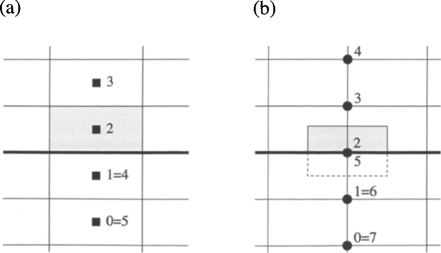
图8.9:坐标切割(粗线):单元中心格式(a),对偶控制体格式(b)。虚单元(点)编号为0和1。
8.8 Periodic Boundaries 周期边界[cfd-8-8]
在某些实际应用中,流场相对于一个或多个坐标方向是周期性的。在这种情况下,只需在其中一个重复区域内模拟流动即可,而与其余物理域的正确相互作用则通过周期边界条件来保证。en
There are certain practical applications where the flow field is periodic with respect to one or multiple coordinate directions. In such a case, it is sufficient to simulate the flow only within one of the repeating regions. The correct interaction with the remaining physical domain is enforced via periodic boundary conditions.
周期边界可以分为两种基本类型。第一种是平移周期性(translational periodicity),即一个周期边界通过纯粹的坐标平移就能变换成另一个边界。第二种类型是由坐标旋转生成的周期边界,因此我们称之为旋转周期性(rotational periodicity)。en
We can distinguish between two basic types of periodic boundaries. The first one covers translational periodicity. This means that one periodic boundary can be transformed into the other boundary by pure coordinate translation. The second type represents periodic boundaries, which were generated by coordinate rotation. Thus, we speak of rotational periodicity.
下面我们将描述单元中心格式和单元顶点格式中周期边界条件的实现,并讨论旋转周期性的情形。关于周期边界处理的更多细节可参见文献[37]、[38]。en
In the following, we shall describe the implementation of the periodic boundary conditions for the cell-centred and the cell-vertex scheme. We shall also consider the case of rotational periodicity. Further details of the treatment of periodic boundaries can be found in Refs. [37], [38].
Cell-Centred Scheme 单元中心格式
利用虚单元概念可以简单地实现周期边界条件。让我们考察图8.10中来自叶轮机械的例子。该构型在竖直方向上是周期的。阴影单元1和2分别位于下部和上部周期边界上。根据周期性条件,第一层虚单元对应于对面周期边界上的边界单元,第二层虚单元与第二层物理单元通信,依此类推。于是,虚单元中所有标量(密度、压力等)都直接取自相应的物理单元,即en
The utilisation of the dummy-cells concept enables a simple implementation of the periodic boundary condition. Let us consider the example from turbomachinery in Fig. 8.10. The configuration is periodic in the vertical direction. The shaded cells 1 and 2 are located on the lower and the upper periodic boundary, respectively. Due to the periodicity condition, the first dummy-cell layer corresponds to the boundary cells at the opposite periodic boundary. The second dummy-cell layer communicates with the second layer of the physical cells and so on. Hence, all scalar quantities (density, pressure, etc.) in the dummy cells are obtained directly from the corresponding physical cells, i.e,
在平移周期性的情形下,同样的关系对向量量(速度、梯度)也成立。旋转周期边界则要求对向量变量作修正,这将在下文进一步讨论。en
The same relations hold also for the vector quantities (velocity, gradients) in the case of translational periodicity. Rotational-periodic boundaries require a correction of the vector variables. This will be discussed further below.
Cell-Vertex Scheme (Dual Control Volume) 单元顶点格式(对偶控制体)
情形如图8.11所示。处理周期边界的一种方法是绕阴影控制体的各个面积分通量,然后把图8.11中点1和点2处的残差相加,以得到完整的净通量,即en
This situation is sketched in Fig. 8.11. One approach for the treatment of periodic boundaries consists of the integration of the fluxes around the faces of the shaded control volumes. The residuals at the points 1 and 2 in Fig. 8.11 are then summed in order to obtain the complete net flux. Thus,
点1和点2处的部分控制体(图8.11中的阴影部分)也必须相加。在平移周期性的情形下,来自对面边界的残差保持不变,即\(\vec{R}_{1'}=\vec{R}_1\)和\(\vec{R}_{2'}=\vec{R}_2\),由此得到\(\vec{R}_{1,sum}=\vec{R}_{2,sum}\)。旋转周期边界则要求先对动量方程作变换,然后才能应用式(8.43)。en
The partial control volumes at the points 1 and 2 (shaded in Fig. 8.11) have to be added up as well. In the case of translational periodicity, the residuals from the opposite boundary remain unchanged, i.e., \(\vec{R}_{1'}=\vec{R}_1\) and \(\vec{R}_{2'}=\vec{R}_2\). This results in \(\vec{R}_{1,sum}=\vec{R}_{2,sum}\). Rotationally periodic boundaries require a transformation of the momentum equations before Eq. (8.43) can be applied.
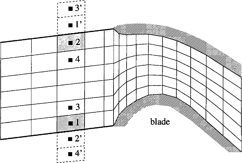
图8.10:二维非结构/结构网格、单元中心格式情形下的周期边界(粗线)。虚单元(虚线)用相应物理单元的(带撇)编号标记。
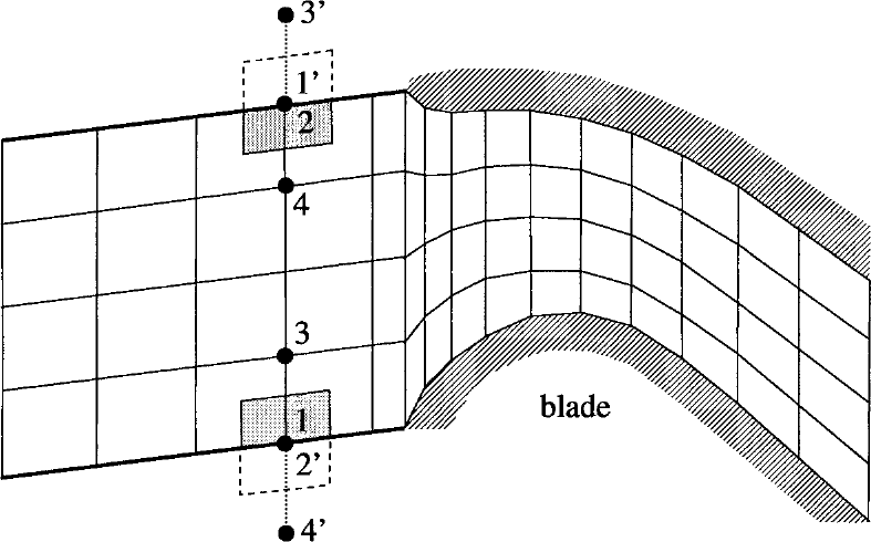
图8.11:二维非结构/结构网格、带对偶控制体的单元顶点格式情形下的周期边界(粗线)。控制体的“虚”部分(虚线)用对面边界上相应控制体的(带撇)编号标记,虚点3'和4'亦同。
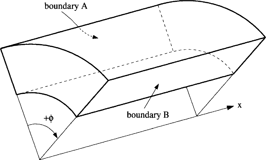
图8.12:旋转周期边界(A与B)。假设旋转轴与\(x\)轴重合。
Rotational Periodicity 旋转周期性
旋转周期条件基于坐标系的旋转。因此,所有向量量(如速度以及标量的梯度)都必须相应地变换;而压力、密度等对坐标旋转不变的标量则保持不变。如果我们假设旋转轴平行于\(x\)轴(见图8.12),则旋转矩阵为en
The rotational periodicity condition is based on a rotation of the coordinate system. Therefore, all vector quantities like velocity or gradients of scalars have to be transformed accordingly. Scalar quantities like pressure or density, which are invariant with respect to coordinate rotation, remain unchanged. If we assume the rotational axis is parallel to the \(x\)-axis (see Fig. 8.12), the rotation matrix becomes
其中周期边界\(A\)与\(B\)之间的角度\(\phi\)以顺时针方向为正。因此,例如从边界\(A\)变换到边界\(B\)的速度向量(图8.10中的单元\(1'\)、\(2'\),图8.11中的点\(1'\)-\(4'\))为en
where the angle \(\phi\) between the periodic boundaries \(A\) and \(B\) is positive in the clockwise direction. Hence, for example, the velocity vector transformed from boundary \(A\) to \(B\) (cells \(1'\), \(2'\) in Fig. 8.10 and points \(1'\)-\(4'\) in Fig. 8.11) reads
容易证明,\(\vec{v}_A\)的\(x\)分量(即\(u_A\))不因旋转而改变,因此\(u_B=u_A\)。所有流动量的梯度都以类似方式变换。en
It is easy to show that the \(x\)-component of \(\vec{v}_A\) (i.e., \(u_A\)) is not changed by the rotation. Thus, \(u_B=u_A\). The gradients of all flow quantities are transformed in similar way.
8.9 Interface Between Grid Blocks 网格块之间的界面[cfd-8-9]
在第3.1节讨论结构网格的空间离散时我们已经看到,对于几何上复杂的求解域,通常不可能生成单一网格(见图3.4)。我们提到了解决这一问题的两种可行方法:第一种是多块(multiblock)方法,第二种是Chimera技术。下面我们将描述多块方法的基本实现问题。更全面的讨论可参见文献[39]-[45]。文献[46]对多块方法作了非常有帮助的介绍。此处不加讨论的Chimera技术的细节可参见文献[47]-[51]。en
During the discussion of the spatial discretisation with structured grids in Section 3.1, it became evident that it is usually not possible to generate a single grid inside a geometrically complex domain (see Fig. 3.4). We mentioned two possible methodologies how to solve the problem. The first one was the multiblock approach and the second one was the Chimera technique. In the following, we shall describe the basic implementation issues of the multiblock approach. For more throughout discussion, the reader is referred to Refs. [39]-[45]. A very helpful introduction to the multiblock methodology was presented in [46]. Details of the Chimera technique, which is not treated here, can be found in Refs. [47]-[51].
在多块技术中,物理域被分割成一定数目的虚拟部分,计算域也随之被划分成相同数目的块。在一般情形下,某个特定块内的物理解会依赖于一个或多个相邻块中的流动。因此,我们必须提供一种数据结构,使各块之间能够高效地交换信息;如果用不同的处理器求解各网格块中的控制方程,这种结构也是通信所必需的。en
Within the multiblock technique, the physical domain is split into a certain number of virtual parts. Consequently, the computational domain becomes also divided into the same number of blocks. In a general case, the physical solution in a particular block will depend on the flow in one or multiple neighbouring blocks. Therefore, we have to provide a data structure which allows for an efficient exchange of information between the blocks. The structure is also required for communication, if different processors are used to solve the governing equations in the grid blocks.
数据结构的第一部分是块边界的编号。图8.13展示了一种具体的编号方案。图8.13中的编号策略可以归纳如下:en
The first part of the data structure consists of the numbering of the block boundaries. One particular numbering scheme is displayed in Fig. 8.13. The numbering strategy in Fig. 8.13 can be summarised as follows:
重要的是,所有块都要采用同一个编号方案。计算空间中网格点的指标\(i\)、\(j\)、\(k\)定义为如下范围en
It is important that all blocks employ the same numbering scheme. The indices \(i\), \(j\), \(k\) of the grid points in the computational space are defined in the ranges
单元中心格式所需要的单元指标\(I\)、\(J\)、\(K\)以类似的方式定义。由于多块方法通常利用虚单元/点来实现,物理单元/点相对每个范围的起点或终点会有一定的偏移(见图8.1)。en
The cell indices \(I\), \(J\), \(K\), which are required by the cell-centred scheme are defined in a similar way. Since the multiblock approach is usually implemented using dummy cells/points, the physical cells/points will have a certain offset from the start or the end of each range (see Fig. 8.1).
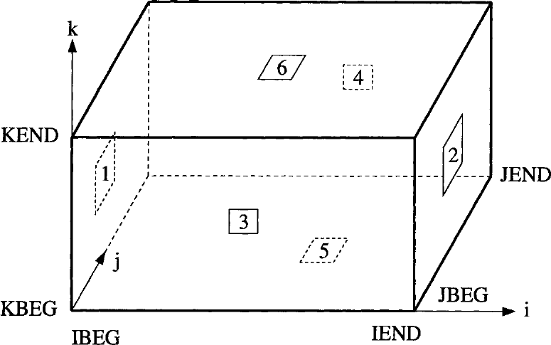
图8.13:计算空间各边及块边界的编号。
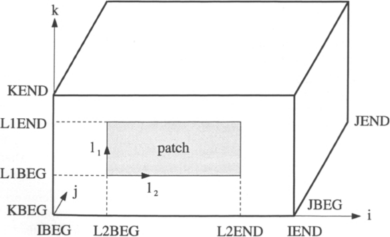
图8.14:计算空间中边界区块(patch)的坐标。区块拥有自己的局部坐标系\(l_1\)、\(l_2\)。
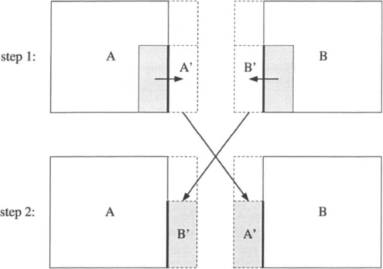
图8.15:两个块A与B之间流动变量的交换。阴影区\(A'\)、\(B'\)为被交换的流动变量;虚层用虚线表示。
每个块的边界被划分为若干互不重叠的区块(patch)。这样就可以在同一块边界上规定不同的边界条件,情形描绘于图8.14。为了唯一地标识每个区块,必须存储相应块的编号和块边界的编号;此外,还必须存储区块的原点、高度和宽度。为此,图8.14中使用了坐标\(L1BEG\)、\(L1END\)、\(L2BEG\)和\(L2END\)。建议按照循环方向(cyclic directions)来定向区块的坐标系:这就是说,如果考虑\(i\)坐标,则\(j\)和\(k\)分别是第一和第二循环方向;对于\(j\)坐标,循环方向则相应变为\(k\)和\(i\)。因此,由于图8.14中的区块位于\(j=JBEG\)边界上,\(l_1\)坐标沿\(k\)方向,\(l_2\)沿\(i\)方向。利用循环方向可以唯一地定义每个区块的取向。en
The boundary of each block is divided into a number of non-overlapping patches. This allows the specification of different boundary conditions on the same block boundary. The situation is depicted in Fig. 8.14. For a unique identification of each patch it is necessary to store the number of the corresponding block and the number of the block boundary. Furthermore, the origin, the height and the width of the patch must be stored. For this purpose, the coordinates \(L1BEG\), \(L1END\), \(L2BEG\) and \(L2END\) are used in Fig. 8.14. It is suggested to orient the coordinate system of the patch according to the cyclic directions. This means, that if we consider the \(i\)-coordinate, \(j\) and \(k\) will be the first and the second cyclic direction. In the case of the \(j\)-coordinate, the cyclic directions will become \(k\) and \(i\), respectively. Therefore, since the patch in Fig. 8.14 is on the \(j=JBEG\) boundary, the \(l_1\)-coordinate is oriented in the \(k\)-direction and \(l_2\) in the \(i\)-direction. The application of the cyclic directions allows for a unique definition of the orientation of each patch.
数据结构的其余部分保证数据能够在那些代表块间界面的区块之间交换(这里我们假设各块只通过其面通信)。为此,需要在上述区块数据结构中补充相邻块与相邻区块的编号;此外,还必须对相互通信的区块彼此之间的取向进行编码。en
The remaining part of the data structure makes sure that data can be exchanged between those patches, which represent interfaces between the blocks (we assume here that the blocks communicate only across their faces). For this purpose, it is required to extend the above patch data structure by the numbers of the adjacent block and patch. It is furthermore necessary to code the orientation of the communicating patches with respect to each other.
两个块之间流动量的交换如图8.15所示。该过程由两步组成。第一步,把域中被相邻区块的虚层所覆盖的那部分区域内的变量写入本块的虚单元/点或临时存储区(图8.15中的\(A'\)和\(B'\));对所有块都执行这一步。第二步,在两个块之间交换\(A'\)和\(B'\)中的数据,也就是说,把\(A'\)写入块B的虚层,把\(B'\)写入块A的虚层。如果两个区块的取向不同,数据必须作相应变换。当网格线在块界面处不对齐时,还需要一些其他操作,如文献[52]、[53]所述。en
The exchange of flow quantities between two blocks is sketched in Fig. 8.15. The procedure consists of two steps. In the first step, variables from the part of the domain, which is overlapped by the dummy layers of the adjacent patch are written to the own dummy cells/points or to a temporary storage (\(A'\) and \(B'\) in Fig. 8.15). This is done for all blocks. In the second step, the data in \(A'\) and \(B'\) is exchanged between both blocks. This means that \(A'\) is written to the dummy layers of block B and \(B'\) to the dummy layers of block A. If the two patches have a different orientation, the data must be transformed accordingly. In cases where the grid lines do not match at the block interface, further operations are required as described, e.g., in [52], [53].
8.10 Flow Gradients at Boundaries of Unstructured Grids 非结构网格边界上的流动梯度[cfd-8-10]
我们在第5.3.4小节中已经指出,对于中位对偶(median-dual)格式,流动梯度的计算需要格外小心。如果在三角形或四面体网格上用式(5.50)的Green-Gauss方法计算梯度,那么来自求解域边界的贡献(对称边界和周期边界除外)必须像式(8.12)或式(8.13)那样计算,而不是取算术平均,否则梯度将不准确。采用图8.4中的记号,边界节点1处的贡献为en
We already stated in Subsection 5.3.4 that the evaluation of the flow gradients requires some care in the case of the median-dual scheme. If the gradients are calculated on triangular or tetrahedral grids using the Green-Gauss approach in Eq. (5.50), the contributions from the boundaries of the domain (except at symmetry or periodic boundaries) must be evaluated similar to Eq. (8.12) or Eq. (8.13), instead of the arithmetic average. Otherwise, the gradient will not be accurate. Considering the notation in Fig. 8.4, the contribution to the boundary node 1 reads
其中\(\Delta S_{123}/3\)是三角形1-2-3中的灰色面积。在混合网格上,更合适的做法是采用带虚拟边的最小二乘法[8](见图5.15)。en
with \(\Delta S_{123}/3\) being the grey area in the triangle 1-2-3. On mixed grids, it is more appropriate to employ the least squares approach with virtual edges [8] (see Fig. 5.15).
单元中心格式在对称边界或周期边界处不需要任何特殊处理,其实现与第8.6节或第8.8节中对通量的讨论完全相同。对于中位对偶格式,如果梯度用最小二乘法计算,情况也是如此。唯一需要额外做的工作是把某些梯度置零,如前面第8.6节所述(参见式(8.40))。en
The cell-centred scheme requires no special provisions at symmetry or periodic boundaries. The implementation is identical to that discussed for the fluxes in Section 8.6 or 8.8. This holds also for the median-dual scheme, if the gradients are evaluated using the least-squares approach. The only additional work required is to set certain gradients to zero as described previously in Section 8.6 (cf. Eq. (8.40)).
如果在中位对偶格式中采用Green-Gauss方法(即应用式(5.50)),就必须修正控制体中触及边界的那些面的法向量(如图8.4中点\(2^{*}\)处):做法是把面向量中所有垂直于对称面的分量置零。最后,梯度按第8.6节所述进行修正。在周期边界处,边界两侧的梯度和体积必须按第8.8节对通量的做法(式(8.43))求和。在旋转周期性的情形下,梯度需要通过应用式(8.44)中的旋转矩阵来变换。en
If the Green-Gauss approach is employed within the median-dual scheme (i.e., if Eq. (5.50) is applied), it is necessary to correct normal vectors of those faces of the control volume, which touch the boundary (like at point \(2^{*}\) in Fig. 8.4). This is done by setting all components of the face vector to zero, which are normal to the symmetry plane. Finally, the gradients are corrected as discussed in Section 8.6. At periodic boundaries, the gradients and the volumes from both sides of the boundary have to be summed up as presented in Section 8.8 for the fluxes (Eq. (8.43)). In the case of rotational periodicity, the gradients needs to be transformed by applying the rotation matrix in Eq. (8.44).