8.7 Coordinate Cut 坐标切割[cfd-8-7]
这种边界条件只在结构网格的情形下遇到。坐标切割(coordinate cut)是人工边界,而非物理边界。它由计算坐标不同但物理位置相同的网格点构成(二维为一条线,三维为一个平面)。这意味着网格被折叠得与自己相接触。正如我们将在第11.1.1小节看到的,坐标切割出现在所谓的C-网格拓扑(图11.5)或O-网格拓扑(图11.9)中。流动变量及其梯度在切割两侧必须保持连续。en
This type of boundary condition is encountered only in the case of structured grids. The coordinate cut represents an artificial, not a physical, boundary. It is a line (plane in 3D) composed of grid points with different computational coordinate(s) but the same physical location. This means that the grid is folded such that it touches itself. As we shall see in Subsection 11.1.1, the coordinate cut appears for the so-called C- (Fig. 11.5) or O-grid topology (Fig. 11.9). The flow variables and their gradients have to stay continuous across the cut.
实现切割边界条件的最好办法是采用虚单元(点)。情形如图8.9所示。可以看到,这里的虚层并不是虚拟的,它们与切割另一侧的网格重合。因此,虚单元(单元中心格式)或虚点(单元顶点格式)中物理量的值直接取自对面的单元(点)。对于单元中心格式,边界单元(图8.9a中的阴影部分)各面上的通量完全像内部流场中那样计算。en
The best way to implement the cut boundary condition is to employ dummy cells (points). The situation is sketched in Fig. 8.9. As we can see, the dummy layers here are not virtual, but they coincide with the grid on the opposite side of the cut. Hence, the values of physical quantities in the dummy cells (cell-centred scheme), or in the dummy points (cell-vertex scheme), are obtained directly from the opposite cells (points). In the case of the cell-centred scheme, the fluxes across the faces of the boundary cell (shaded in Fig. 8.9a) are evaluated exactly like in the interior field.
对于单元顶点格式,切割边界可以用两种不同的方式处理。一种可能是在切割处生成完整的控制体(第二部分在图8.9b中用虚线表示),利用虚点,通量可以像域内一样计算。如果实现正确,点2(上网格部分)与点5(下部分)处的流动量将相等。第二种方法是对控制体的每一半分别积分通量,然后把图8.9b中点2和点5处的残差相加。重要的是,点2和点5处的部分控制体也必须求和。en
The cut boundary can be treated in two different ways for the cell-vertex scheme. One possibility is to generate a complete control volume at the cut (the second part is denoted by a dashed line in Fig. 8.9b). Using the dummy points, the fluxes can be calculated in the same way as inside the domain. If the implementation is done correctly, the flow quantities at the points 2 (upper grid part) and 5 (lower part) will be equal. The second approach is to integrate the fluxes separately for each half of the control volume. The residuals at the points 2 and 5 in Fig. 8.9b are then added. It is important that the partial control volumes at the points 2 and 5 are summed up as well.
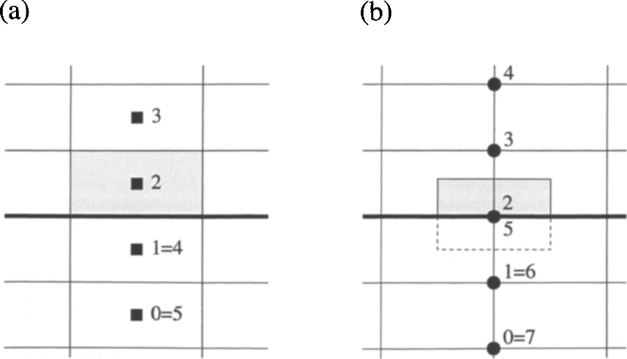
图8.9:坐标切割(粗线):单元中心格式(a),对偶控制体格式(b)。虚单元(点)编号为0和1。