8.2.1 Inviscid Flow 无黏流动[cfd-8-2-1]

对于无黏流动，流体在表面上滑移。由于不存在摩擦力，速度矢量必定与表面相切。这等价于没有沿表面法向流动的条件，即en

In the case of an inviscid flow, the fluid slips over the surface. Since there is no friction force, the velocity vector must be tangent to the surface. This is equivalent to the condition that there is no flow normal to the surface, i.e.,

\vec{v}\cdot\vec{n}=0\quad\text{at the surface}, \tag{8.1}

其中 $\vec{n}$ 表示表面处的单位法向量。因此，逆变速度 $$V$$ （式(2.22)）在壁面上为零。于是，对流通量向量式(2.21)只剩下压力项，即en

where $\vec{n}$ denotes the unit normal vector at the surface. Hence, the contravariant velocity $$V$$ (Eq. (2.22)) is zero at the wall. Consequently, the vector of convective fluxes Eq. (2.21) reduces to the pressure term alone, i.e,

(\vec{F}_c)_w=\begin{bmatrix} 0\\ n_x\,p_w\\ n_y\,p_w\\ n_z\,p_w\\ 0 \end{bmatrix} \tag{8.2}

其中 $$p_w$$ 为壁面压力。en

with $$p_w$$ being the wall pressure.

Structured Cell-Centred Scheme 结构化单元中心格式

在单元中心格式中，压力在单元的形心处求值。然而，式(8.2)中的 $$p_w$$ 却需要取在边界单元的面上。最简便的做法是由域内外推得到壁面压力。参见图8.2，我们可以简单地取 $$p_w=p_2$$ 。若采用两点公式en

Within the cell-centred scheme, the pressure is evaluated at the centroid of the cell. However, $$p_w$$ in Eq. (8.2) is required at the face of the boundary cell. We can obtain the wall pressure most easily by extrapolation from the interior of the domain. Considering Fig. 8.2, we could simply set $$p_w=p_2$$ . Higher accuracy is achieved by using either a two-point

p_w=\frac{1}{2}\left(3p_2-p_3\right), \tag{8.3}

或三点外推公式en

or a three-point extrapolation formula

p_w=\frac{1}{8}\left(15p_2-10p_3+3p_4\right). \tag{8.4}

为了计及网格拉伸的影响，可以用到壁面的距离来代替其中的常数系数[1]。en

In order to account for grid stretching, distances to the wall could be employed instead of the constant coefficients [1].

上述外推公式(8.3)、(8.4)没有考虑网格与表面几何。另一种方法——所谓的法向动量关系（normal-momentum relation）——由Rizzi提出[2]。它基于这样一个事实：在无黏流动中壁面代表一条流线。把式(8.1)的法向零流动条件沿表面流线求导，并将结果代入动量方程，便得到en

The above extrapolation formulae (8.3), (8.4) do not account for the grid and the surface geometry. An alternative approach - the so-called normal-momentum relation - was developed by Rizzi [2]. It is based on the fact that the wall represents a streamline in inviscid flow. Differentiation of the zero-normal-flow condition in Eq. (8.1) along the surface streamline, and the substitution of the result into the momentum equation yields

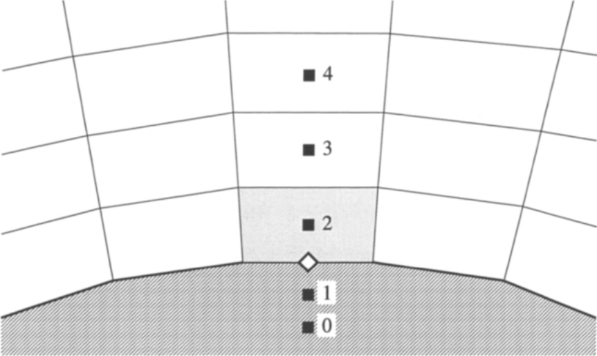
\rho\vec{v}\cdot\left(\vec{v}\cdot\vec{\nabla}\right)\vec{n}=\vec{n}\cdot\vec{\nabla}p\,. \tag{8.5}

图8.2:单元中心格式的固壁边界条件

图8.2:单元中心格式的固壁边界条件。虚单元记为0和1。计算对流通量式(8.2)的位置用菱形标记。

图8.3:结构化单元顶点对偶控制体格式的固壁边界条件

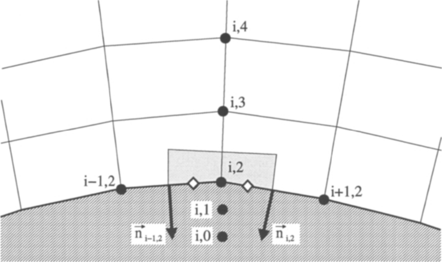
图8.3:结构化单元顶点对偶控制体格式的固壁边界条件。虚点记为(i,0)和(i,1)。计算对流通量式(8.2)的位置用菱形标出。另请对照图4.6中的示意。

式(8.5)把密度、速度和壁面几何与压力的法向导数联系起来。已经证明，法向动量关系能给出非常精确的结果[1]。然而，在复杂几何情形下，法向动量关系的数值求解可能出现问题。实现的详细描述与精度比较见文献[1]。en

Equation (8.5) relates the density, the velocity and the wall geometry to the normal derivative of the pressure. It was demonstrated that the normal-momentum relation gives very accurate results [1]. However, problems can arise with the numerical solution of the normal-momentum relation in the case of complex geometries. Detailed description of the implementation and accuracy comparisons can be found in Ref. [1].

虚单元中守恒变量的取值可以由域内线性外推得到，即en

The values of the conservative variables in the dummy cells can be obtained by linear extrapolation from the interior, i.e.,

\begin{aligned} \vec{W}_1&=2\vec{W}_2-\vec{W}_3\\ \vec{W}_0&=3\vec{W}_2-2\vec{W}_3\,. \end{aligned} \tag{8.6}

式(8.6)中的下标与图8.2对应。如果要在空间离散格式中使用虚单元（例如计算耗散算子），重要的是对流通量的计算要与式(8.2)相容。en

The indices in Eq. (8.6) correspond to Fig. 8.2. If the dummy cells are to be utilised within the spatial discretisation scheme (e.g., for the evaluation of the dissipation operator), it is important that the calculation of the convective fluxes is compatible to Eq. (8.2).

Structured Cell-Vertex Scheme 结构化单元顶点格式

对于具有重叠控制体的单元顶点离散格式（小节4.2.2），边界条件式(8.1)的实现很直接。壁面上的对流通量按式(8.2)计算。壁面压力 $$p_w$$ 通过节点值平均得到：二维情形如式(4.26)所示，三维情形如式(4.27)所示。分布公式（二维为式(4.30)）此时只涉及两个（三维为四个）单元（请比较图4.4与图8.3）。en

The implementation of the boundary condition Eq. (8.1) is straightforward for the cell-vertex discretisation scheme with overlapping control volumes (Subsection 4.2.2). The convective fluxes at the wall faces are computed according to Eq. (8.2). The wall pressure $$p_w$$ is obtained by averaging the nodal values as indicated in Eq. (4.26) for a 2-D, or in Eq. (4.27) for a 3-D case. The distribution formula (Eq. (4.30) in 2D) accounts now for only two (four in 3D) cells (compare Fig. 4.4 to Fig. 8.3).

对于具有对偶控制体的单元顶点格式（小节4.2.3），可以采用几种不同的做法。一种做法是对位于壁面上的控制体的每个面分别应用式(8.2)中的条件。于是，按照图8.3，可以写出en

Several different ways can be followed in the case of the cell-vertex scheme with dual control volumes (Subsection 4.2.3). One approach is to apply the condition in Eq. (8.2) separately for each face of the control volume which is on the wall. Thus, according to Fig. 8.3, we can write

(\vec{F}_{c,w})_{i,2}=\begin{bmatrix} 0\\ (n_x)_{i-1,2}\,(p_w)_{i-1/4,2}\\ (n_y)_{i-1,2}\,(p_w)_{i-1/4,2}\\ (n_z)_{i-1,2}\,(p_w)_{i-1/4,2}\\ 0 \end{bmatrix}+\begin{bmatrix} 0\\ (n_x)_{i,2}\,(p_w)_{i+1/4,2}\\ (n_y)_{i,2}\,(p_w)_{i+1/4,2}\\ (n_z)_{i,2}\,(p_w)_{i+1/4,2}\\ 0 \end{bmatrix}. \tag{8.7}

式(8.7)中的压力 $(p_w)_{i-1/4,2}$ 和 $(p_w)_{i+1/4,2}$ 可通过线性插值得到，例如en

The pressures $(p_w)_{i-1/4,2}$ and $(p_w)_{i+1/4,2}$ in Eq. (8.7) can be obtained by linear interpolation, e.g.,

(p_w)_{i+1/4,2}=\frac{1}{4}\left[3(p_w)_{i,2}+(p_w)_{i+1,2}\right]. \tag{8.8}

相应的三维公式将在后面非结构网格小节中给出。en

The corresponding 3-D formula will be presented further below in the subsection on unstructured grids.

另一种可行做法是直接在相应壁面节点处（即图8.3中的节点 $$(i,2)$$ ）应用式(8.2)中的条件。壁面压力 $$p_w$$ 直接取为 $p_{i,2}$ 。单位法向量取为共享节点 $$(i,2)$$ 的所有壁面小面（facet）法向量的平均。这一做法需要对速度矢量作修正：在用时间推进格式更新解之后，把壁面上的速度矢量投影到切平面上[3]、[4]，即en

Another possible implementation employs the condition in Eq. (8.2) directly in the respective wall node (i.e., node $$(i,2)$$ in Fig. 8.3). The wall pressure $$p_w$$ is simply set equal to $p_{i,2}$ . The unit normal vector is computed as the average of the normal vectors of all wall facets which share the node $$(i,2)$$ . This approach requires a correction of the velocity vector. After the solution update by the time-stepping scheme, the velocity vector at the wall is projected onto the tangential plane [3], [4], i.e.,

(\vec{v}_{i,2})_{corr}=\vec{v}_{i,2}-\left[\vec{v}_{i,2}\cdot(\vec{n}_{av})_{i,2}\right]\cdot(\vec{n}_{av})_{i,2} \tag{8.9}

其中 $\vec{n}_{av}$ 为平均后的单位法向量。这样，流动将与壁面相切。en

with $\vec{n}_{av}$ being the averaged unit normal vector. In this way, the flow will become tangential to the wall.

为给虚点赋值，只需用与式(8.6)类似的关系，把守恒变量（式(2.20)）从内场外推即可。en

In order to assign values to the dummy points, it is sufficient to extrapolate the conservative variables (Eq. (2.20)) from the interior field by using a relation similar to Eq. (8.6).

Unstructured Cell-Centred Scheme 非结构单元中心格式

式(8.1)的壁面边界条件在非结构单元中心格式中的实现方式与结构网格类似。如果边界单元是四边形、六面体或棱柱（壁面为三角形的面），可以用式(8.3)把压力外推到壁面。相邻单元（图8.2中的3号单元）可由小节5.2.1所述的基于面的数据结构得到。对于三角形或四面体单元，文献[5]和[6]建议采用一层虚单元，虚单元中的速度分量通过把边界单元的速度矢量关于壁面反射得到。例如，在图8.2中的虚单元1内，速度变为en

The wall boundary condition in Eq. (8.1) can be implemented for a cell-centred unstructured scheme in a way similar to that on structured grids. If the boundary cell is a quadrilateral, hexahedron or a prism (with triangular face on the wall), the pressure can be extrapolated to the wall by using Eq. (8.3). The neighbouring cell (number 3 in Fig. 8.2) is known from the face-based data structure described in Subsection 5.2.1. For the case of a triangular or tetrahedral cell, in Ref. [5] and [6] it was suggested to employ one layer of dummy cells. The velocity components in the dummy cells were obtained by reflecting the velocity vectors in the boundary cells at the wall. For example, in the dummy cell 1 in Fig. 8.2, the velocity would become

\vec{v}_1=\vec{v}_2-2V_2\,\vec{n}\,, \tag{8.10}

其中 $$V_2=u_2n_x+v_2n_y+w_2n_z$$ 为逆变速度， $\vec{n}=[n_x,n_y,n_z]^T$ 表示壁面单位法向量。虚单元中的压力和密度取为与相应边界单元中的值相等（这意味着 $$p_w=p_2$$ ）。en

where $$V_2=u_2n_x+v_2n_y+w_2n_z$$ is the contravariant velocity and $\vec{n}=[n_x,n_y,n_z]^T$ stands for the wall unit-normal vector. The pressure and density in the dummy cells were set equal to the values in the corresponding boundary cell (this implies $$p_w=p_2$$ ).

Unstructured Median-Dual Scheme 非结构中位对偶格式

在非结构中位对偶（median-dual）离散格式的情形下，边界条件式(8.1)需要更多的注意。二维情形如图8.4所示，三维情形如图8.5所示。式(8.2)的对流通量在位于壁面上的控制体每个面处分别计算。这与上文针对具有对偶控制体的结构化单元顶点格式讨论的第一种做法相同。对于四边形元素（如图8.4中的1-3-4-5），压力按与式(8.8)相应的方式插值。对于六面体、棱柱或棱锥，其控制体面为四边形（如图8.5中的面1-4-5-6），插值公式为en

The boundary condition Eq. (8.1) requires more attention in the case of the median-dual unstructured discretisation scheme. The situation is shown in Fig. 8.4 for the 2-D and in Fig. 8.5 for the 3-D case. The convective fluxes in Eq. (8.2) are computed separately at each face of the control volume which is located on the wall. This is identical to the first approach discussed above for the structured cell-vertex scheme with dual control volumes. For quadrilateral elements (like 1-3-4-5 in Fig. 8.4), the pressure is interpolated correspondingly to Eq. (8.8). In the case of hexahedra, prisms or pyramids, where the face of the control volume is a quadrilateral (like face 1-4-5-6 in Fig. 8.5), the interpolation formula reads

p_w=\frac{1}{16}\left(9p_1+3p_4+3p_6+p_5\right). \tag{8.11}

如果边界元素是四面体或棱柱（二维情形为三角形），壁面上的压力应当按有限元方法计算en

If the boundary elements are tetrahedra or prisms (or triangles in 2-D), the pressure at the wall face should be evaluated like in the finite element method

图8.4:二维非结构对偶控制体混合网格格式的固壁边界条件

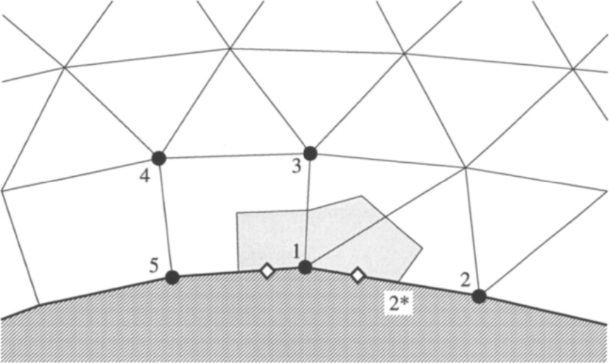
图8.4:二维非结构对偶控制体混合网格格式的固壁边界条件。计算对流通量式(8.2)的位置用菱形标出。

图8.5:三维非结构混合网格格式的固壁边界条件

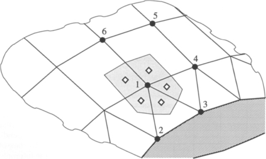
图8.5:三维非结构混合网格格式的固壁边界条件。计算对流通量式(8.2)的位置用菱形标出。

[7]。例如，对于图8.4中的壁面段1-2，面1-2*上的压力应按下式计算en

[7]. At the wall segment 1-2 in Fig. 8.4 for example, the pressure at the face 1-2* would be computed as

p_w=\frac{1}{6}\left(5p_1+p_2\right). \tag{8.12}

对于四面体，例如图8.5中的壁面1-2-3，压力按下式计算en

In the case of a tetrahedra with, e.g., the wall face 1-2-3 in Fig. 8.5, the pressure is evaluated as

p_w=\frac{1}{8}\left(6p_1+p_2+p_3\right). \tag{8.13}

应当强调，这种有限元型插值对获得准确的流动解十分重要[7]。en

It should be stressed that this finite-element type interpolation is important for an accurate flow solution [7].