8.9 Interface Between Grid Blocks 网格块之间的界面[cfd-8-9]
在第3.1节讨论结构网格的空间离散时我们已经看到,对于几何上复杂的求解域,通常不可能生成单一网格(见图3.4)。我们提到了解决这一问题的两种可行方法:第一种是多块(multiblock)方法,第二种是Chimera技术。下面我们将描述多块方法的基本实现问题。更全面的讨论可参见文献[39]-[45]。文献[46]对多块方法作了非常有帮助的介绍。此处不加讨论的Chimera技术的细节可参见文献[47]-[51]。en
During the discussion of the spatial discretisation with structured grids in Section 3.1, it became evident that it is usually not possible to generate a single grid inside a geometrically complex domain (see Fig. 3.4). We mentioned two possible methodologies how to solve the problem. The first one was the multiblock approach and the second one was the Chimera technique. In the following, we shall describe the basic implementation issues of the multiblock approach. For more throughout discussion, the reader is referred to Refs. [39]-[45]. A very helpful introduction to the multiblock methodology was presented in [46]. Details of the Chimera technique, which is not treated here, can be found in Refs. [47]-[51].
在多块技术中,物理域被分割成一定数目的虚拟部分,计算域也随之被划分成相同数目的块。在一般情形下,某个特定块内的物理解会依赖于一个或多个相邻块中的流动。因此,我们必须提供一种数据结构,使各块之间能够高效地交换信息;如果用不同的处理器求解各网格块中的控制方程,这种结构也是通信所必需的。en
Within the multiblock technique, the physical domain is split into a certain number of virtual parts. Consequently, the computational domain becomes also divided into the same number of blocks. In a general case, the physical solution in a particular block will depend on the flow in one or multiple neighbouring blocks. Therefore, we have to provide a data structure which allows for an efficient exchange of information between the blocks. The structure is also required for communication, if different processors are used to solve the governing equations in the grid blocks.
数据结构的第一部分是块边界的编号。图8.13展示了一种具体的编号方案。图8.13中的编号策略可以归纳如下:en
The first part of the data structure consists of the numbering of the block boundaries. One particular numbering scheme is displayed in Fig. 8.13. The numbering strategy in Fig. 8.13 can be summarised as follows:
重要的是,所有块都要采用同一个编号方案。计算空间中网格点的指标\(i\)、\(j\)、\(k\)定义为如下范围en
It is important that all blocks employ the same numbering scheme. The indices \(i\), \(j\), \(k\) of the grid points in the computational space are defined in the ranges
单元中心格式所需要的单元指标\(I\)、\(J\)、\(K\)以类似的方式定义。由于多块方法通常利用虚单元/点来实现,物理单元/点相对每个范围的起点或终点会有一定的偏移(见图8.1)。en
The cell indices \(I\), \(J\), \(K\), which are required by the cell-centred scheme are defined in a similar way. Since the multiblock approach is usually implemented using dummy cells/points, the physical cells/points will have a certain offset from the start or the end of each range (see Fig. 8.1).
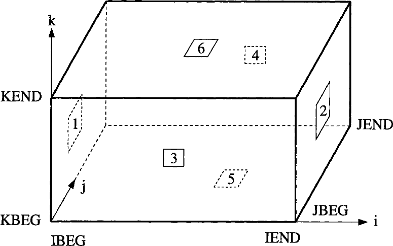
图8.13:计算空间各边及块边界的编号。
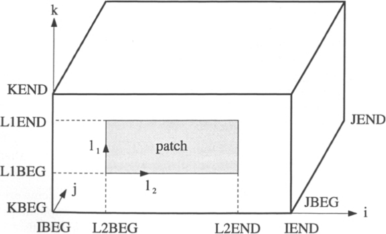
图8.14:计算空间中边界区块(patch)的坐标。区块拥有自己的局部坐标系\(l_1\)、\(l_2\)。
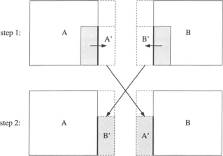
图8.15:两个块A与B之间流动变量的交换。阴影区\(A'\)、\(B'\)为被交换的流动变量;虚层用虚线表示。
每个块的边界被划分为若干互不重叠的区块(patch)。这样就可以在同一块边界上规定不同的边界条件,情形描绘于图8.14。为了唯一地标识每个区块,必须存储相应块的编号和块边界的编号;此外,还必须存储区块的原点、高度和宽度。为此,图8.14中使用了坐标\(L1BEG\)、\(L1END\)、\(L2BEG\)和\(L2END\)。建议按照循环方向(cyclic directions)来定向区块的坐标系:这就是说,如果考虑\(i\)坐标,则\(j\)和\(k\)分别是第一和第二循环方向;对于\(j\)坐标,循环方向则相应变为\(k\)和\(i\)。因此,由于图8.14中的区块位于\(j=JBEG\)边界上,\(l_1\)坐标沿\(k\)方向,\(l_2\)沿\(i\)方向。利用循环方向可以唯一地定义每个区块的取向。en
The boundary of each block is divided into a number of non-overlapping patches. This allows the specification of different boundary conditions on the same block boundary. The situation is depicted in Fig. 8.14. For a unique identification of each patch it is necessary to store the number of the corresponding block and the number of the block boundary. Furthermore, the origin, the height and the width of the patch must be stored. For this purpose, the coordinates \(L1BEG\), \(L1END\), \(L2BEG\) and \(L2END\) are used in Fig. 8.14. It is suggested to orient the coordinate system of the patch according to the cyclic directions. This means, that if we consider the \(i\)-coordinate, \(j\) and \(k\) will be the first and the second cyclic direction. In the case of the \(j\)-coordinate, the cyclic directions will become \(k\) and \(i\), respectively. Therefore, since the patch in Fig. 8.14 is on the \(j=JBEG\) boundary, the \(l_1\)-coordinate is oriented in the \(k\)-direction and \(l_2\) in the \(i\)-direction. The application of the cyclic directions allows for a unique definition of the orientation of each patch.
数据结构的其余部分保证数据能够在那些代表块间界面的区块之间交换(这里我们假设各块只通过其面通信)。为此,需要在上述区块数据结构中补充相邻块与相邻区块的编号;此外,还必须对相互通信的区块彼此之间的取向进行编码。en
The remaining part of the data structure makes sure that data can be exchanged between those patches, which represent interfaces between the blocks (we assume here that the blocks communicate only across their faces). For this purpose, it is required to extend the above patch data structure by the numbers of the adjacent block and patch. It is furthermore necessary to code the orientation of the communicating patches with respect to each other.
两个块之间流动量的交换如图8.15所示。该过程由两步组成。第一步,把域中被相邻区块的虚层所覆盖的那部分区域内的变量写入本块的虚单元/点或临时存储区(图8.15中的\(A'\)和\(B'\));对所有块都执行这一步。第二步,在两个块之间交换\(A'\)和\(B'\)中的数据,也就是说,把\(A'\)写入块B的虚层,把\(B'\)写入块A的虚层。如果两个区块的取向不同,数据必须作相应变换。当网格线在块界面处不对齐时,还需要一些其他操作,如文献[52]、[53]所述。en
The exchange of flow quantities between two blocks is sketched in Fig. 8.15. The procedure consists of two steps. In the first step, variables from the part of the domain, which is overlapped by the dummy layers of the adjacent patch are written to the own dummy cells/points or to a temporary storage (\(A'\) and \(B'\) in Fig. 8.15). This is done for all blocks. In the second step, the data in \(A'\) and \(B'\) is exchanged between both blocks. This means that \(A'\) is written to the dummy layers of block B and \(B'\) to the dummy layers of block A. If the two patches have a different orientation, the data must be transformed accordingly. In cases where the grid lines do not match at the block interface, further operations are required as described, e.g., in [52], [53].