chapter. Turbulence Modelling 第7章 湍流建模[cfd-0008]
与层流相反,湍流的突出特征是分子沿复杂而不规则的路径以混乱的方式运动。强烈的混乱运动使流体的各个层强烈地混合在一起。由于分子与固体壁面之间的动量和能量交换增强,在相同条件下,湍流导致的壁面摩擦和传热都比层流更高。en
The outstanding feature of a turbulent flow, in the opposite to a laminar flow, is that the molecules move in a chaotic fashion along complex irregular paths. The strong chaotic motion causes the various layers of the fluid to mix together intensely. Because of the increased momentum and energy exchange between the molecules and solid walls, turbulent flow leads at the same conditions to higher skin friction and heat transfer as compared to laminar flow.
尽管流动变量的混沌脉动具有确定性的本质,湍流的模拟至今仍是一个重大难题。尽管现代超级计算机性能强大,但利用含时的Navier-Stokes方程(2.19)对湍流进行直接模拟——即所谓直接数值模拟(Direct Numerical Simulation,DNS)[1]–[10]——只适用于雷诺数(\(Re\))在\(10^4-10^5\)量级的较为简单的流动问题。DNS之所以未能得到更广泛的应用,是因为要获得足够的空间分辨率,所需网格点数按\(Re^{9/4}\)标度,而CPU时间按\(Re^3\)标度。因此,我们不得不以近似的方式计及湍流的影响。为此,人们发展了种类繁多的湍流模型,相关研究至今仍在继续。湍流模型有五个主要类别:
- 代数模型;
- 一方程模型;
- 多方程模型;
- 二阶封闭(雷诺应力模型);
- 大涡模拟(Large-Eddy Simulation,LES)。
en
Although the chaotic fluctuations of the flow variables are of deterministic nature, the simulation of turbulent flows still continues to present a significant problem. Despite the performance of modern supercomputers, a direct simulation of turbulence by the time-dependent Navier-Stokes equations (2.19) -- known as the Direct Numerical Simulation (DNS) [1]--[10] -- is applicable only to relatively simple flow problems at low Reynolds numbers (\(Re\)) in the order of \(10^4-10^5\). A more widespread utilisation of the DNS is prevented by the fact that the number of grid points needed for sufficient spatial resolution scales as \(Re^{9/4}\) and the CPU-time as \(Re^3\). Therefore, we are forced to account for the effects of turbulence in an approximate manner. For this purpose, a large variety of turbulence models was developed and the research still goes on. There are five principal classes of turbulence models:
- algebraic,
- one-equation,
- multiple-equation,
- second-order closures (Reynolds-stress models),
- Large-Eddy Simulation (LES).
前三类模型属于所谓的一阶封闭(first-order closures)。它们主要基于Boussinesq的涡黏性假设[11]、[12],但对某些应用也基于非线性涡黏性表述。图7.1给出了按复杂程度递减排序的各类湍流模型的概览。en
The first tree models belong to the so-called first-order closures. They are based mostly on the eddy-viscosity hypothesis of Boussinesq [11], [12], but for certain applications also on non-linear eddy-viscosity formulations. An overview of the classes of turbulence models, which are sorted according to their decreasing level of complexity, is displayed in Fig. 7.1.
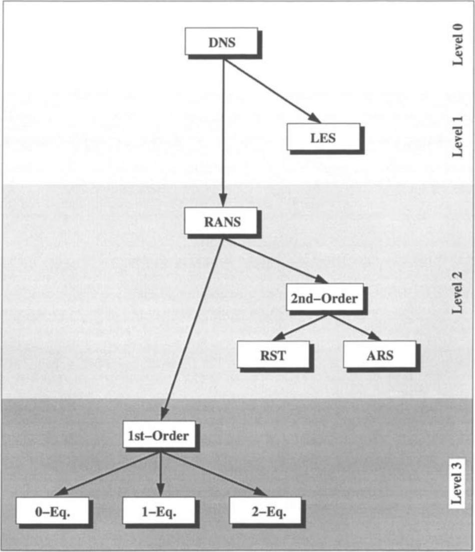
图7.1:湍流模型的层级。缩写:DNS——直接数值模拟(Direct Numerical Simulation);LES——大涡模拟(Large-Eddy Simulation);RANS——雷诺平均Navier-Stokes方程(Reynolds-Averaged Navier-Stokes equations);1st-order——一阶封闭(first-order closures);2nd-order——二阶封闭(second-order closures);RST——雷诺应力输运模型(Reynolds-Stress Transport models);ARS——代数雷诺应力模型(Algebraic Reynolds-Stress models);0-、1-、2-Eq.——零方程(代数)、一方程、两方程模型。
应当意识到,不存在能够可靠预测所有类型湍流的单一湍流模型。每种模型都有其长处和短处。例如,某个模型如果在附着边界层的情形下工作得很好,它对分离流动则可能完全失效。因此,始终应当问一问:该模型是否包含了所研究流动的全部重要特征。此外还应考虑的一点是计算量与特定应用所需精度之间的权衡。我们的意思是,在许多情况下,数值上廉价的湍流模型预测某些全局量所能达到的精度,与更复杂的模型相同。en
One should be aware of the fact that there is no single turbulence model, which can predict reliably all kinds of turbulent flows. Each of the models has its strengths and weaknesses. For example, if a particular model works perfectly in the case of attached boundary layers, it may fail completely for separated flows. Thus, it is important always to ask whether the model includes all the significant features of the flow being investigated. Another point which should be taken into consideration is the computational effort versus the accuracy required by the particular application. We mean by this that in many cases a numerically inexpensive turbulence model can predict some global measures with the same accuracy as a more complex model.
下面,我们先介绍对控制方程作时间平均和质量平均而得到的湍流基本方程。然后,我们介绍Boussinesq涡黏性方法和非线性涡黏性方法。随后,我们简要讨论雷诺应力输运方程,它构成代数和微分雷诺应力模型的基础。在7.2节中,我们介绍几种广泛使用的一方程和两方程一阶封闭。最后,由于工程应用日益增多,我们将较为详细地讨论LES及相关方法。en
In the following, we first introduce the basic equations of turbulence as they result from time and mass averaging of the governing equations. Then, we present the Boussinesq's and the non-linear eddy-viscosity approaches. After that, we briefly discuss the Reynolds-stress transport equation, which forms the basis of the algebraic and differential Reynolds-stress models. In Section 7.2, we present few wide-spread one- and two-equation first-order closures. Finally, we discuss LES and related approaches in some detail because of the growing number of engineering applications.
7.1 Basic Equations of Turbulence 湍流的基本方程[cfd-7-1]
首先,让我们把控制方程(2.19)改写成微分形式(见附录A.1),因为湍流建模文献中经常使用这种形式;此外,它还使记号紧凑而清晰。不过,我们也会给出湍流方程积分形式的例子。en
First of all, let us rewrite the governing equations (2.19) in differential form (see Appendix A.1), since this is used very often in literature on turbulence modelling. Furthermore, it allows for a compact and clear notation. However, we will also provide examples of turbulence equations in integral form.
对于可压缩Newton流体,在无源项的情形下,Navier-Stokes方程按坐标不变量形式写为en
In the case of a compressible Newtonian fluid, the Navier-Stokes equations read in the absence of source terms in coordinate invariant formulation as
在上述方程(7.1)中,\(v_i\)表示一个速度分量(\(\vec{v}=\left[v_1,v_2,v_3\right]^T\)),\(x_i\)代表一个坐标方向。关于紧凑张量记号的说明见附录A.13。en
In above Eq. (7.1), \(v_i\) denotes a velocity component (\(\vec{v}=\left[v_1,v_2,v_3\right]^T\)), and \(x_i\) stands for a coordinate direction, respectively. An explanation of the compact tensor notation can be found in Appendix A.13.
其中利用了Stokes假设(式(2.17))。在直角坐标系下,式(7.2)与式(2.15)等价。式(7.2)中的第二项,即\(\partial v_k/\partial x_k\),对应于速度的散度,在不可压缩流动中为零。应变率张量(strain-rate tensor)的分量由下式给出en
where we utilised the Stokes's hypothesis (Eq. (2.17)). In Cartesian coordinates, Eq. (7.2) is equivalent to Eq. (2.15). The second term in Eq. (7.2), i.e., \(\partial v_k/\partial x_k\), which corresponds to the divergence of the velocity, disappears for incompressible flows. The components of the strain-rate tensor are given by
与此同时,让我们再定义旋转率张量(rotation-rate tensor,即速度梯度张量的反对称部分),其分量为en
In this connection, let us also define the rotation-rate tensor (antisymmetric part of the velocity gradient tensor) with the following components
它们在直角坐标系中分别对应于式(2.6)和式(2.12)。en
which correspond in Cartesian coordinate system to Eq. (2.6) and Eq. (2.12), respectively.
其中\(\nu=\mu/\rho\)为运动黏性系数,\(\nabla^2\)表示拉普拉斯算子。在没有浮力效应时,温度\(T\)的方程与质量守恒方程和动量方程解耦。en
with \(\nu=\mu/\rho\) being the kinematic viscosity coefficient and \(\nabla^2\) denoting the Laplace operator. In the absence of buoyancy effects, the equation for the temperature \(T\) becomes decoupled from the mass conservation and momentum equations.
7.1.1 Reynolds Averaging 雷诺平均[cfd-7-1-1]
对湍流进行近似处理的第一种方法由Reynolds于1895年提出。该方法基于把流动变量分解为平均值与脉动值两部分。随后求解控制方程(7.1)的平均值——平均值对工程应用最有意义。这样,首先考虑不可压缩流动,方程(7.1)中的速度分量和压力用下式替代[13]en
The first approach for the approximate treatment of turbulent flows was presented by Reynolds in 1895. The methodology is based on the decomposition of the flow variables into a mean and a fluctuating part. The governing equations (7.1) are then solved for the mean values, which are the most interesting for engineering applications. Thus, considering first incompressible flows, the velocity components and the pressure in Eq. (7.1) are substituted by [13]
其中平均值用上划线表示,湍流脉动用撇号表示。平均值通过平均过程求得。雷诺平均(Reynolds averaging)有三种不同的形式:en
where the mean value is denoted by an overbar and the turbulent fluctuations by a prime. The mean values are obtained by an averaging procedure. There are three different forms of the Reynolds averaging:
1. 时间平均(time averaging)——适用于定常湍流(统计定常湍流)en
1. Time averaging -- appropriate for stationary turbulence (statistically steady turbulence)
其结果是,平均值\(\bar{v}_i\)不随时间变化,而只随空间变化。情形如图7.2所示。实践中,\(T\to\infty\)意味着时间间隔\(T\)应远大于湍流脉动的典型时间尺度。en
As a consequence, the mean value \(\bar{v}_i\) does not vary in time, but only in space. The situation is sketched in Fig. 7.2. In practice, \(T\to\infty\) means that the time interval \(T\) should be large as compared to the typical time-scale of the turbulent fluctuations.
2. 空间平均(spatial averaging)——适用于均匀湍流en
2. Spatial averaging -- appropriate for homogeneous turbulence
其中\(\Omega\)为控制体。此时\(\bar{v}_i\)在空间上均匀,但允许随时间变化。en
with \(\Omega\) being a control volume. In this case, \(\bar{v}_i\) is uniform in space, but it is allowed to vary in time.
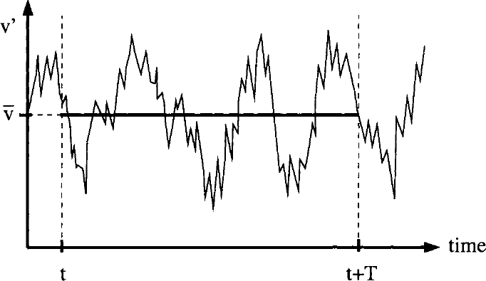
图7.2:雷诺平均——湍流速度脉动\(v'\)与统计平均值\(\bar{v}\)的示意图。
3. 系综平均(ensemble averaging)——适用于一般湍流en
3. Ensemble averaging -- appropriate for general turbulence
这里,平均值\(\bar{v}_i\)仍然是时间和空间坐标的函数。en
Here, the mean value \(\bar{v}_i\) still remains a function of time and of space coordinates.
对所有这三种方法,脉动部分的平均值都为零,即\(\overline{v'_i}=0\)。然而,容易看出\(\overline{v'_iv'_i}\neq 0\)。若两个湍流速度分量相关,则对\(\overline{v'_iv'_j}\)同样如此。en
For all three approaches, the average of the fluctuating part is zero, i.e., \(\overline{v'_i}=0\). However, it can be easily seen that \(\overline{v'_iv'_i}\neq 0\). The same is true for \(\overline{v'_iv'_j}\), if both turbulent velocity components are correlated.
当湍流既是定常的又是均匀的时候,三种平均形式彼此等价。这称为各态历经假设(ergodic hypothesis)。en
In cases where the turbulent flow is both stationary and homogeneous, all three averaging forms are equivalent. This is called the ergodic hypothesis.
7.1.2 Favre (Mass) Averaging Favre(质量)平均[cfd-7-1-2]
在密度不为常数的情形下,对方程(7.1)中的某些量,宜采用密度(质量)加权即Favre分解[14]、[15]来代替雷诺平均。否则,由于出现涉及密度脉动的额外关联,平均后的控制方程会变得复杂得多。最方便的做法是:对密度和压力采用雷诺平均,对速度、内能、焓和温度等其他变量采用Favre平均。Favre平均量(例如速度分量)由如下关系求得[14]、[15]en
In cases where the density is not constant, it is advisable to apply the density (mass) weighted or Favre decomposition [14], [15] to certain quantities in Eq. (7.1) instead of Reynolds averaging. Otherwise, the averaged governing equations would become considerably more complicated due to additional correlations involving density fluctuations. The most convenient way is to employ Reynolds averaging for density and pressure, and Favre averaging for other variables such as velocity, internal energy, enthalpy and temperature. Favre averaged quantities, for example the velocity components, are obtained from the relation [14], [15]
其中\(\bar{\rho}\)表示雷诺平均密度。于是,Favre分解写为en
where \(\bar{\rho}\) denotes the Reynolds-averaged density. Hence, the Favre decomposition reads
其中\(\tilde{v}_i\)表示平均值,\(v''_i\)表示速度\(v_i\)的脉动部分。同样,脉动部分的平均值为零,即\(\widetilde{v''_i}=0\)。此外,若两个脉动量相关,则其乘积的平均值不为零。例如,\(\widetilde{v''_iv''_i}\neq 0\),并且一般地\(\widetilde{v''_iv''_j}\neq 0\)。en
where \(\tilde{v}_i\) represents the mean value and \(v''_i\) the fluctuating part of the velocity \(v_i\). Again, the average of the fluctuating part is zero, i.e., \(\widetilde{v''_i}=0\). Furthermore, the average of the product of two fluctuating quantities is not zero, if the quantities are correlated. Hence, for example, \(\widetilde{v''_iv''_i}\neq 0\) and in general \(\widetilde{v''_iv''_j}\neq 0\).
对于Favre平均与雷诺平均的混合使用,可以导出如下关系en
The following relationships can be derived for a mix between Favre and Reynolds averaging
这些关系将在后面的小节中用到。en
These relations will be utilised in later subsections.
7.1.3 Reynolds-Averaged Navier-Stokes Equations 雷诺平均Navier-Stokes方程[cfd-7-1-3]
雷诺应力张量在三维情形下由九个分量组成en
The Reynolds-stress tensor consists in 3D of the nine components
不过,由于关联中的\(v'_i\)与\(v'_j\)可以互换,雷诺应力张量只包含六个独立分量。各法向应力之和除以密度即定义为湍动能(turbulent kinetic energy),即en
However, since \(v'_i\) and \(v'_j\) in the correlations can be interchanged, the Reynolds-stress tensor contains only six independent components. The sum of the normal stresses divided by density defines the turbulent kinetic energy, i.e.,
如我们所见,基于雷诺平均Navier-Stokes方程的湍流建模,其根本问题在于找出六个附加关系式,以使方程(7.14)封闭。我们将在7.1.5–7.1.7小节中介绍基本方法。en
As we can see, the fundamental problem of turbulence modelling based on the Reynolds-averaged Navier-Stokes equations is to find six additional relations in order to close the equations (7.14). We shall introduce the basic methodologies in the Subsections 7.1.5--7.1.7.
7.1.4 Favre- and Reynolds-Averaged Navier-Stokes Equations Favre平均与雷诺平均Navier-Stokes方程[cfd-7-1-4]
在湍流建模中,通常假设Morkovin假设[16]成立。该假设指出:若\(\rho'\ll\bar{\rho}\),边界层的湍流结构不会受到密度脉动的显著影响。对于壁面约束流动,直到马赫数约为5这一结论一般都成立。然而,对于高超声速流动或可压缩自由剪切层,则必须计及密度脉动。对于有燃烧或有显著传热的流动,情况也是如此。en
In turbulence modelling, it is quite common to assume that Morkovin's hypothesis [16] is valid. It states that the turbulent structure of a boundary layer is not notably influenced by density fluctuations if \(\rho'\ll\bar{\rho}\). This is generally true for wall-bounded flows up to a Mach number of about five. However, in the case of hypersonic flows or for compressible free shear layers, density fluctuations have to be taken into account. The same holds also for flows with combustion or with significant heat transfer.
这就是Favre平均与雷诺平均Navier-Stokes方程。与雷诺平均类似,动量(和能量)方程中的黏性应力张量要再加上Favre平均雷诺应力张量,即en
These are the Favre- and Reynolds-Averaged Navier-Stokes equations. Similarly to the Reynolds averaging, the viscous stress tensor in the momentum (and energy) equation is extended by the Favre-averaged Reynolds-stress tensor, i.e.,
如果采用Favre平均湍动能的定义,即en
If we employ the definition of the Favre-averaged turbulent kinetic energy, i.e.,
总焓定义为en
The total enthalpy is defined as
Favre平均与雷诺平均Navier-Stokes方程(7.19)的各个部分具有如下物理意义[17]:
- \(\dfrac{\partial}{\partial x_j}\left(k\dfrac{\partial\tilde{T}}{\partial x_j}\right)\)——热的分子扩散
- \(\dfrac{\partial}{\partial x_j}\left(\bar{\rho}\widetilde{v''_jh''}\right)\)——热的湍流输运
- \(\dfrac{\partial}{\partial x_j}\left(\widetilde{\tau_{ij}v''_i}\right)\)——\(\tilde{K}\)的分子扩散
- \(\dfrac{\partial}{\partial x_j}\left(\bar{\rho}\widetilde{v''_jK}\right)\)——\(\tilde{K}\)的湍流输运
- \(\dfrac{\partial}{\partial x_j}\left(\tilde{v}_i\bar{\tau}_{ij}\right)\)——分子应力做的功
- \(\dfrac{\partial}{\partial x_j}\left(\tilde{v}_i\tau^F_{ij}\right)\)——Favre平均雷诺应力做的功
en
The individual parts of the Favre- and Reynolds-averaged Navier-Stokes equations (7.19) have the following physical meaning [17]:
- \(\dfrac{\partial}{\partial x_j}\left(k\dfrac{\partial\tilde{T}}{\partial x_j}\right)\) - molecular diffusion of heat
- \(\dfrac{\partial}{\partial x_j}\left(\bar{\rho}\widetilde{v''_jh''}\right)\) - turbulent transport of heat
- \(\dfrac{\partial}{\partial x_j}\left(\widetilde{\tau_{ij}v''_i}\right)\) - molecular diffusion of \(\tilde{K}\)
- \(\dfrac{\partial}{\partial x_j}\left(\bar{\rho}\widetilde{v''_jK}\right)\) - turbulent transport of \(\tilde{K}\)
- \(\dfrac{\partial}{\partial x_j}\left(\tilde{v}_i\bar{\tau}_{ij}\right)\) - work done by the molecular stresses
- \(\dfrac{\partial}{\partial x_j}\left(\tilde{v}_i\tau^F_{ij}\right)\) - work done by the Favre-averaged Reynolds stresses
\(\tilde{K}\)的分子扩散和湍流输运在很多时候都可以忽略。对于跨声速和超声速流动,这是有效的近似。为使Favre平均与雷诺平均方程(7.19)封闭,还必须提供Favre平均雷诺应力张量(式(7.20))的六个分量以及湍流热通量向量的三个分量。我们将在后面几个小节中讨论这三种基本方法。en
The molecular diffusion and turbulent transport of \(\tilde{K}\) are very often neglected. This is a valid approximation for transonic and supersonic flows. In order to close the Favre- and Reynolds-averaged equations (7.19), we also have to supply six components of the Favre-averaged Reynolds-stress tensor (Eq. (7.20)) and three components of the turbulent heat-flux vector. We shall discuss the three basic approaches in the next subsections.
7.1.5 Eddy-Viscosity Hypothesis 涡黏性假设[cfd-7-1-5]
湍流建模领域最重要的贡献之一由Boussinesq于1877年作出[11]、[12]。他的想法基于如下观察:湍流中的动量输运由大而高能的湍流涡所引起的混合主导。Boussinesq假设湍流剪应力像层流中那样线性地依赖于平均应变率,其比例系数就是涡黏性(eddy viscosity)。对于雷诺平均不可压缩流动(式(7.14)),Boussinesq假设可以写为en
One of the most significant contributions to turbulence modelling was presented in 1877 by Boussinesq [11], [12]. His idea is based on the observation that the momentum transfer in a turbulent flow is dominated by the mixing caused by large energetic turbulent eddies. The Boussinesq hypothesis assumes that the turbulent shear stress depends linearly on the mean rate of strain, as in a laminar flow. The proportionality factor is the eddy viscosity. The Boussinesq hypothesis for Reynolds averaged incompressible flow (Eq. (7.14)) can be written as
其中\(\overline{S}_{ij}\)表示雷诺平均应变率张量(式(7.3),另见式(7.16)),\(K\)为湍动能(\(K=(1/2)\overline{v'_iv'_i}\)),\(\mu_T\)代表涡黏性。与分子黏性\(\mu\)不同,涡黏性\(\mu_T\)不是流体的物理特性,而是局部流动条件的函数。此外,\(\mu_T\)还受到流动历史效应的强烈影响。en
where \(\overline{S}_{ij}\) denotes the Reynolds-averaged strain-rate tensor (Eq. (7.3), cf. also Eq. (7.16)), \(K\) is the turbulent kinetic energy (\(K=(1/2)\overline{v'_iv'_i}\)), and \(\mu_T\) stands for the eddy viscosity. Unlike the molecular viscosity \(\mu\), the eddy viscosity \(\mu_T\) represents no physical characteristic of the fluid, but it is a function of the local flow conditions. Additionally, \(\mu_T\) is also strongly affected by flow history effects.
其中\(\tilde{S}_{ij}\)和\(\tilde{K}\)分别为Favre平均应变率和Favre平均湍动能。注意它与式(7.2)的相似性。式(7.24)和(7.25)中的\((2/3)\rho K\delta_{ij}\)项是为了得到\(\tau^R_{ij}\)或\(\tau^F_{ij}\)的正确迹(trace)所必需的。这意味着,我们必须有en
where \(\tilde{S}_{ij}\) and \(\tilde{K}\) are the Favre-averaged strain rate and turbulent kinetic energy, respectively. Note the similarity to Eq. (7.2). The term \((2/3)\rho K\delta_{ij}\) in Eqs. (7.24) and (7.25) is required in order to obtain the proper trace of \(\tau^R_{ij}\) or \(\tau^F_{ij}\). This means that we must have
即在\(\overline{S}_{ii}=0\)(连续方程)或\(\tilde{S}_{ii}=0\)的情形下,以满足湍动能的关系式(7.18)或(7.21)。然而,\((2/3)\rho K\delta_{ij}\)这一项常常被忽略,特别是在与较简单的湍流模型(如代数模型)联用时。en
in the case of \(\overline{S}_{ii}=0\) (continuity equation) or \(\tilde{S}_{ii}=0\), in order to fulfil the relations Eq. (7.18) or (7.21) for the turbulent kinetic energy. However, the term \((2/3)\rho K\delta_{ij}\) is often neglected, particularly in connection with simpler turbulence models (like algebraic ones).
对湍流热通量向量建模时常用的近似基于经典的Reynolds比拟[18]。于是,我们可以写en
The approximation, which is commonly used for the modelling of the turbulent heat-flux vector, is based on the classical Reynolds analogy [18]. Hence, we may write
其中湍流热导率系数(turbulent thermal conductivity coefficient)\(k_T\)定义为en
with the turbulent thermal conductivity coefficient \(k_T\) being defined as
在方程(7.27)中,\(c_p\)表示定压比热系数,\(Pr_T\)为湍流Prandtl数。一般假设湍流Prandtl数在整个流场中为常数(对空气\(Pr_T=0.9\))。en
In Equation (7.27), \(c_p\) denotes the specific heat coefficient at constant pressure and \(Pr_T\) is the turbulent Prandtl number. The turbulent Prandtl number is in general assumed to be constant over the flow field (\(Pr_T=0.9\) for air).
把涡黏性方法应用于控制方程(2.19)或方程(7.1)的雷诺(及Favre)平均形式时,黏性应力张量式(2.15)或式(7.2)中的动力黏性系数\(\mu\)被简单地替换为层流分量与湍流分量之和,即en
By applying the eddy-viscosity approach to the Reynolds- (and Favre-) averaged form of the governing equations (2.19) or Eq. (7.1), the dynamic viscosity coefficient \(\mu\) in the viscous stress tensor Eq. (2.15) or Eq. (7.2) is simply replaced by the sum of a laminar and a turbulent component, i.e.,
至少从工程的角度看,Boussinesq的涡黏性概念非常有吸引力,因为它“只”需要确定\(\mu_T\)(式(7.24)或(7.25)中\((2/3)\rho K\delta_{ij}\)项所需的湍动能\(K\),或者作为湍流模型的副产物得到,或者干脆略去)。一旦知道了涡黏性\(\mu_T\),通过引入平均流动变量并把\(\mu_T\)加到层流黏性上,我们就能容易地把Navier-Stokes方程(2.19)或(7.1)扩展用于湍流模拟。因此,Boussinesq方法成为了大量一阶湍流封闭的基础。然而,对某些应用而言,Boussinesq假设不再成立(例如见[17]第214页或[19]第111页):
- 平均应变率发生突然变化的流动;
- 具有显著流线曲率的流动;
- 具有旋转和分层的流动;
- 管道和透平机械中的二次流;
- 边界层分离与再附的流动。
en
The eddy-viscosity concept of Boussinesq is, at least from the engineering point of view, very attractive since it requires ``only'' the determination of \(\mu_T\) (the turbulent kinetic energy \(K\) needed for the term \((2/3)\rho K\delta_{ij}\) in Eq. (7.24) or (7.25) is either obtained as a by-product of the turbulence model or is simply omitted). Once we know the eddy viscosity \(\mu_T\), we can easily extend the Navier-Stokes equations (2.19) or (7.1) to the simulation of turbulent flows by introducing averaged flow variables and by adding \(\mu_T\) to the laminar viscosity. Therefore, Boussinesq's approach became the basis for a large variety of first-order turbulence closures. However, there are applications for which the Boussinesq hypothesis is no longer valid (see, e.g., [17] p. 214 or [19] p. 111):
- flows with sudden change of mean strain rate,
- flows with significant streamline curvature,
- flows with rotation and stratification,
- secondary flows in ducts and in turbomachinery,
- flows with boundary layer separation and reattachment.
涡黏性方法的局限源于把湍流与平均应变场视为处于平衡状态的假设,以及其结果与系统旋转无关的假定。通过在湍流模型中加入适当的修正项,结果可以明显改善[20]、[21]。采用下面要介绍的非线性涡黏性模型,可以进一步提高预测精度。en
The limitations of the eddy-viscosity approach are caused by the assumption of equilibrium between the turbulence and the mean strain field, as well as by the independence on system rotation. The results can be notably improved by using appropriate correction terms in the turbulence models [20], [21]. Further increased accuracy of predictions can be achieved through the application of non-linear eddy-viscosity models which are described next.
7.1.6 Non-Linear Eddy Viscosity 非线性涡黏性[cfd-7-1-6]
为了消除湍流与平均应变率之间平衡假设所强加的限制,Lumley[22]、[23]提议用应变张量与旋转张量的高阶乘积来扩展线性的Boussinesq方法。这可以视为一种Taylor级数展开。沿着Lumley的思路,人们提出了众多非线性涡黏性模型,例如文献[24]–[29]。en
In order to remove the restrictions imposed by the assumption of equilibrium between the turbulence and the mean strain rate, Lumley [22], [23] proposed to extend the linear Boussinesq approach by higher-order products of strain and rotation tensors. This can viewed as a Taylor series expansion. Following the idea of Lumley, numerous non-linear eddy-viscosity models were proposed, see, for example, Refs. [24]--[29].
下面我们介绍由Shih等人[25]提出的一种较新的方法。它在一般涡黏性表述中包含直至三阶的项,特别适合于旋转流(swirling flows)。正如文献[19]第194页所指出的,三次项对高精度至关重要。雷诺应力\(\tau^R_{ij}\)可以表示为[25]、[30](对照式(7.24))en
In the following, we shall present one recent approach proposed by Shih et al. [25]. It includes up to third-order terms in the general eddy-viscosity formulation and is particularly suited to swirling flows. As already pointed out in [19], p. 194, cubic terms are essential for high accuracy. The Reynolds stresses \(\tau^R_{ij}\) can be expressed as [25], [30] (cf. Eq. (7.24))
湍动能\(K\)和耗散率(dissipation rate)\(\varepsilon\)的值由低雷诺数\(K\)-\(\varepsilon\)湍流模型给出(参见7.2.2小节)。式(7.30)中的系数\(C_1\)至\(C_5\)见文献[25]、[30]。en
The values of the turbulent kinetic energy \(K\) and the dissipation rate \(\varepsilon\) are obtained from low-Reynolds \(K\)-\(\varepsilon\) turbulence model (cf. Subsection 7.2.2). The factors \(C_1\) to \(C_5\) in Eq. (7.30) are provided in Refs. [25], [30].
与线性涡黏性方法相比,非线性模型的计算代价只略微增大,但对复杂湍流的预测能力却有显著提高。en
In comparison to the linear eddy-viscosity approach, the non-linear models are computationally only slightly more expensive, but they offer a substantially improved prediction capabilities for complex turbulent flows.
7.1.7 Reynolds-Stress Transport Equation 雷诺应力输运方程[cfd-7-1-7]
通过取时间平均(二阶矩),可以为雷诺应力导出精确方程en
It is possible to derive exact equations for the Reynolds stresses by taking the time average (second-order moment)
其中\(\mathcal{N}(v_i)\)表示Navier-Stokes算子,即en
where \(\mathcal{N}(v_i)\) denotes the Navier-Stokes operator, i.e.,
它适用于不可压缩流动。可压缩流动的表述见文献[17]第179页,或[32]、[33]。方程(7.34)中,湍动能的生成项\(P_{ij}\)、压力—应变项\(\Pi_{ij}\)、耗散率项\(\varepsilon_{ij}\)以及三阶扩散项\(C_{ijk}\)定义为en
for incompressible flow. The formulation for compressible flows can be found in Ref. [17], p. 179, or in [32], [33]. The production of the turbulent kinetic energy \(P_{ij}\), the pressure-strain term \(\Pi_{ij}\), the dissipation-rate term \(\varepsilon_{ij}\), and the third-order diffusion term \(C_{ijk}\) in Eq. (7.34) are defined as
在方程(7.35)中,\(S'_{ij}\)表示应变率张量的脉动部分。\(C_{ijk}\)的第一部分(三重速度项)表示由脉动对流驱动的输运,另外两部分则分别是压力输运项(压力—速度关联)。en
In Eq. (7.35), \(S'_{ij}\) denotes the fluctuating part of the strain-rate tensor. The first part of \(C_{ijk}\), the triple velocity term, represents transport driven by fluctuating convection, the two other parts are the pressure transport terms (pressure-velocity correlations), respectively.
如我们所见,精确的雷诺应力方程包含新的未知高阶关联(例如\(\overline{v'_iv'_jv'_k}\))。因此,方程(7.34)只能借助经验模型来封闭。这是由Navier-Stokes方程的非线性本质造成的。二阶封闭——雷诺应力模型——为求解方程(7.34)提供了必要的框架。实施的例子可参见文献[34]–[36]。en
As we can see, the exact Reynolds-stress equation contains new unknown higher-order correlations (e.g., \(\overline{v'_iv'_jv'_k}\)). Therefore, Equation (7.34) can be closed only by using empirical models. This is caused by the non-linear nature of the Navier-Stokes equations. The second-order closures -- the Reynolds-stress models -- provide the necessary framework for solving Eq. (7.34). Examples of implementations can be found, e.g., in Refs. [34]--[36].
7.2 First-Order Closures 一阶封闭[cfd-7-2]
一阶封闭(first-order closures)是在雷诺/Favre平均Navier-Stokes方程中近似雷诺应力的最简单方法。它们基于Boussinesq涡黏性模型或非线性涡黏性模型,我们分别在小节7.1.5和7.1.6中讨论过。因此,相应湍流建模的任务就是计算涡黏性\(\mu_T\)。en
The first-order closures represent the easiest way to approximate the Reynolds stresses in the Reynolds-/Favre-averaged Navier-Stokes equations. They are based on Boussinesq or non-linear eddy-viscosity models, which we discussed in the Subsections 7.1.5 and 7.1.6, respectively. Consequently, the task of an associated turbulence model is to compute the eddy viscosity \(\mu_T\).
从种类繁多的一阶封闭模型中,我们选出了三种广泛使用、代表当前技术水平的方法。这三种模型都可以方便地在结构网格和非结构网格上实现。首先,我们讨论Spalart和Allmaras提出的单方程模型;其次,我们介绍著名的K-\(\varepsilon\)双方程模型;最后,我们考察由Menter提出的K-\(\omega\) SST(剪切应力输运,Shear-Stress Transport)双方程模型。关于这些湍流模型在各种算例下的详细比较可参见[37]。en
From the large variety of first-order closure models, we selected three widely-used approaches which represent the current state-of-the-art. All three models can be implemented easily on structured as well as on unstructured grids. First, we shall discuss the one-equation model due to Spalart and Allmaras. Second, we shall present the well-known K-\(\varepsilon\) two-equation model. Finally, we shall consider the K-\(\omega\) SST (Shear-Stress Transport) two-equation model proposed by Menter. A detailed comparison of this turbulence models for various cases can be found in [37].
在下文中,密度和速度分量都应理解为雷诺平均/Favre平均量,只是为简便起见省略了相应的记号。en
In the following, the density and the velocity components should be understood as Reynolds-/Favre-averaged, although the corresponding notation is omitted for convenience.
7.2.1 Spalart-Allmaras One-Equation Model Spalart-Allmaras 单方程模型[cfd-7-2-1]
Spalart-Allmaras单方程湍流模型[38]对涡黏性变量\(\tilde{\nu}\)求解输运方程。它是在经验、量纲分析和伽利略不变性的基础上发展起来的,并利用二维混合层、尾流和平板边界层的结果进行了标定。Spalart-Allmaras模型还能对具有逆压梯度的湍流流动给出相当准确的预测。此外,它能够在用户指定的位置实现从层流到湍流的平滑转捩。Spalart-Allmaras模型具有若干良好的数值特性:它是“局部的”,即某一点处的方程不依赖于其他点上的解,因此可以方便地在结构多块网格或非结构网格上实现;它还稳健、向定态收敛快,并且近壁区域只需适中的网格分辨率。en
The Spalart-Allmaras one-equation turbulence model [38] employs transport equation for an eddy-viscosity variable \(\tilde{\nu}\). It was developed based on empiricism, dimensional analysis and Galilean invariance. It was calibrated using results for 2-D mixing layers, wakes and flat-plate boundary layers. The Spalart-Allmaras model also allows for reasonably accurate predictions of turbulent flows with adverse pressure gradients. Furthermore, it is capable of smooth transition from laminar to turbulent flow at user specified locations. The Spalart-Allmaras model has several favourable numerical features. It is "local" which means that the equation at one point does not depend on the solution at other points. Therefore, it can be readily implemented on structured multi-block or on unstructured grids. It is also robust, converges fast to steady-state and requires only moderate grid resolution in the near-wall region.
Differential Form 微分形式
Spalart-Allmaras湍流模型用张量记号可以写成如下形式[38]en
The Spalart-Allmaras turbulence model can be written in tensor notation as follows [38]
右端各项分别代表涡黏性生成、守恒性扩散、非守恒性扩散、近壁湍流破坏、生成的转捩阻尼以及湍流的转捩源。此外,\(\nu_L = \mu_L/\rho\)表示层流运动黏度,\(d\)为到最近壁面的距离(壁面距离的计算见文献[39])。式(7.28)和(7.29)中的湍流涡黏性由下式得到en
The terms on the right-hand side represent eddy-viscosity production, conservative diffusion, non-conservative diffusion, near-wall turbulence destruction, transition damping of production, and transition source of turbulence. Furthermore, \(\nu_L = \mu_L/\rho\) denotes the laminar kinematic viscosity and \(d\) is the distance to the closest wall (for the computation of wall distances see Ref. [39]). The turbulent eddy viscosity in Eq. (7.28) and (7.29) is obtained from
生成项用下列公式求值en
The production term is evaluated with the following formulae
其中\(\Omega_{ij}\)由式(7.4)给出。注意\(\tilde{S}\)与文献[38]中的原始定义不同,这一修改是Spalart提出的,目的是防止\(\tilde{S}\)变为零(参见文献[40],第155页)。en
where \(\Omega_{ij}\) is given by Eq. (7.4). Note that \(\tilde{S}\) differs from its original definition in [38]. The modification was suggested by Spalart in order to prevent \(\tilde{S}\) from reaching zero (cf. Ref. [40], p. 155).
控制涡黏性破坏的项为en
The terms controlling the destruction of the eddy viscosity read
用于模拟层流-湍流转捩的函数为en
Functions used for modelling the laminar-turbulent transition are given by
其中\(\omega_t\)表示转捩触发点(trip point,位置须由用户指定)处壁面上的涡量,\(\|\Delta\vec{v}\|_2\)表示触发点速度与当前流场点速度之差的2-范数,\(d_t\)为到最近触发点的距离,\(\Delta x_t\)表示触发点处沿壁面的网格间距。en
where \(\omega_t\) represents the vorticity at the wall at the trip point (position has to be specified by the user), \(\|\Delta\vec{v}\|_2\) denotes the 2-norm of the difference between the velocity at the trip point and the current field point, \(d_t\) is the distance to the nearest trip point, and \(\Delta x_t\) stands for the spacing along the wall at the trip point.
为了考虑非平衡效应对生成项的影响,最近有文献提出把\(C_{b1}\)表示为应变率的函数[41]。en
In order to account for non-equilibrium effects on the production term, it was recently proposed to express \(C_{b1}\) as a function of the strain rate [41].
用下面的表达式来代替en
by the following expression
这样就可以避开对项\(\left(\partial\tilde{\nu}/\partial x_j\right)^2\)做离散化的困难。en
In this way, difficulties with the discretisation of the term \(\left(\partial\tilde{\nu}/\partial x_j\right)^2\) are circumvented.
Integral Form 积分形式
其中\(\Omega\)表示控制体,\(\partial\Omega\)为其表面,\(dS\)是\(\Omega\)的面元。对流通量定义为en
where \(\Omega\) represents the control volume, \(\partial\Omega\) its surface, and \(dS\) is a surface element of \(\Omega\). The convective flux is defined as
其中\(V\)为逆变速度(见式(2.22))。对流通量一般用一阶上风格式离散。黏性通量为en
with \(V\) being the contravariant velocity (see Eq. (2.22)). The convective flux is in general discretised using a first-order upwind scheme. The viscous flux is given by
其中\(n_x\)、\(n_y\)和\(n_z\)是单位法向量的分量。法向黏性应力为en
where \(n_x\), \(n_y\), and \(n_z\) are the components of the unit normal vector. The normal viscous stresses read
Initial and Boundary Conditions 初始条件与边界条件
\(\tilde{\nu}\)的初值通常取\(\tilde{\nu} = 0.1\,\nu_L\)。入口边界上也指定同样的值。在出口边界上,\(\tilde{\nu}\)直接由计算域内部外推。在固体壁面上,宜取\(\tilde{\nu} = 0\),从而\(\mu_T = 0\)。en
The initial value of \(\tilde{\nu}\) is usually taken as \(\tilde{\nu} = 0.1\,\nu_L\). The same value is also specified at inflow boundaries. At outflow boundaries, \(\tilde{\nu}\) is simply extrapolated from the interior of the computational domain. At solid walls, it is appropriate to set \(\tilde{\nu} = 0\) and hence \(\mu_T = 0\).
7.2.2 K-ε Two-Equation Model K-ε 双方程模型[cfd-7-2-2]
K-\(\varepsilon\)湍流模型是应用最广泛的双方程涡黏性模型。它基于对湍动能\(K\)和湍流耗散率\(\varepsilon\)的方程求解。K-\(\varepsilon\)模型的历史渊源可以追溯到周培源的工作[42]。20世纪70年代期间,该模型的多种形式被提出,其中最重要的贡献来自Jones和Launder[43]、[44],Launder和Sharma[45],以及Launder和Spalding[46]。en
The K-\(\varepsilon\) turbulence model is the most widely employed two-equation eddy-viscosity model. It is based on the solution of equations for the turbulent kinetic energy \(K\) and the turbulent dissipation rate \(\varepsilon\). The historic roots of the K-\(\varepsilon\) model reach to the work of Chou [42]. During the 1970's, various formulations of the model were proposed. The most important contributions were due to Jones and Launder [43], [44], Launder and Sharma [45] as well as due to Launder and Spalding [46].
K-\(\varepsilon\)湍流模型需要加入所谓的阻尼函数(damping functions),才能在黏性底层内一直有效直至壁面。阻尼函数的目的是保证\(K\)和\(\varepsilon\)在壁面处具有正确的极限行为,即en
The K-\(\varepsilon\) turbulence model requires addition of the so-called damping functions in order to stay valid through the viscous sublayer to the wall. The aim of the damping functions is to assure proper limiting behaviour of \(K\) and \(\varepsilon\) at the wall, i.e.,
其中\(y\)表示垂直于壁面的坐标。此外还可以证明,雷诺剪切应力在近壁处的行为如(参见例如[17],第138-139页)en
where \(y\) represents the coordinate normal to the wall. Further, it can be shown that the Reynolds shear stress behaves like (see, e.g., [17] pp. 138-139)
带阻尼函数的K-\(\varepsilon\)模型也被称为低雷诺数(low Reynolds number)模型。使用最广泛的阻尼函数形式由Jones和Launder[43]、Launder和Sharma[45]、Lam和Bremhorst[47]以及Chien[48]提出。七种不同的低雷诺数K-\(\varepsilon\)模型的比较可在文献[49]中找到。en
The K-\(\varepsilon\) models with damping functions are also denoted as low Reynolds number models. The most widely used formulations of the damping functions were proposed by Jones and Launder [43], Launder and Sharma [45], Lam and Bremhorst [47], and by Chien [48]. The reader may find a comparison of seven different low Reynolds number K-\(\varepsilon\) models in Ref. [49].
K-\(\varepsilon\)湍流模型在数值求解上比前述Spalart-Allmaras模型(小节7.2.1)更困难。特别是,阻尼函数使湍流方程带有刚性源项。这一点,加上壁面附近为解析黏性底层所必需的高网格分辨率,要求至少采用点隐式、最好采用全隐式的时间推进格式。文献[50]给出了关于K-\(\varepsilon\)方程显式时间离散的有用提示。K-\(\varepsilon\)模型在结构网格和非结构网格上实现的例子可参见例如[51]-[59]。最后,需要特别指出,对于具有逆压梯度的流动,K-\(\varepsilon\)模型的精度会下降[49]、[17]。en
The K-\(\varepsilon\) turbulence model is more difficult to solve numerically than the previously discussed Spalart-Allmaras model (Subsection 7.2.1). Particularly, the damping functions lead to turbulence equations with stiff source terms. This, and the necessary high grid resolution nearby walls (in order to resolve the viscous sublayer), requires the utilisation of at least point-implicit or better full-implicit time-stepping schemes. Reference [50] contains useful hints on the explicit time discretisation of the K-\(\varepsilon\) equations. Examples of implementations of the K-\(\varepsilon\) model on structured as well as on unstructured grids can be found, e.g., in [51]-[59]. Finally, it is important to note that the accuracy of the K-\(\varepsilon\) model degrades for flows with adverse pressure gradient [49], [17].
Differential Form 微分形式
一个低雷诺数K-\(\varepsilon\)模型可以写成en
A low Reynolds number K-\(\varepsilon\) model can be written as
右端各项分别代表守恒性扩散、涡黏性生成和耗散。此外,\(\phi_{\varepsilon}\)表示所谓的显式壁面项。Favre平均湍流应力\(\tau_{ij}^F\)由式(7.25)给出,应变率张量\(S_{ij}\)由式(7.3)得到。式(7.28)和(7.29)中的湍流涡黏性由下式求得en
The terms on the right-hand side represent conservative diffusion, eddy-viscosity production and dissipation, respectively. Furthermore, \(\phi_{\varepsilon}\) denotes the so-called explicit wall term. The Favre-averaged turbulent stresses \(\tau_{ij}^F\) are given by Eq. (7.25) and the strain-rate tensor \(S_{ij}\) follows from Eq. (7.3). The turbulent eddy viscosity in Eq. (7.28) and (7.29) results from
按式(7.24)或式(7.25)计算涡黏性时也要用到湍动能。量\(\varepsilon^{*}\)与湍流耗散率\(\varepsilon\)通过下式相联系en
The turbulent kinetic energy is also employed for the evaluation of the eddy viscosity according to Eq. (7.24) or Eq. (7.25). The quantity \(\varepsilon^{*}\) is related to the turbulent dissipation rate \(\varepsilon\) by
在不同的K-\(\varepsilon\)模型中,常数、近壁阻尼函数以及壁面项各不相同。这里我们选择Launder-Sharma模型,因为它在很宽的应用范围内都给出良好结果[49]。对Launder-Sharma模型,常数和湍流Prandtl数为[45]en
The constants, the near-wall damping functions as well as the wall term differ between the various K-\(\varepsilon\) models. Here, we choose the Launder-Sharma model because it gives good results for a wide range of applications [49]. For the Launder-Sharma model, the constants and the turbulent Prandtl number are given by [45]
此外,近壁阻尼函数为en
Furthermore, the near-wall damping functions read
其中\(Re_T = \rho K^2/(\varepsilon^{*}\mu_L)\)为湍流雷诺数。(译注:\(f_{\varepsilon2}\)中的指数项原书印作\(\exp(Re_T^2)\),无负号;按Launder–Sharma模型的通行形式应为\(\exp(-Re_T^2)\),疑为原书排印疏漏,此处照录原书。)en
with \(Re_T = \rho K^2/(\varepsilon^{*}\mu_L)\) being the turbulent Reynolds number.
最后,显式壁面项\(\phi_{\varepsilon}\)和\(\varepsilon_w\)的值定义为en
Finally, the explicit wall term \(\phi_{\varepsilon}\) and the value \(\varepsilon_w\) are defined as
其中\(v_s\)表示平行于壁面的速度,\(y_n\)表示垂直于壁面的坐标。为了避免显式地知道壁面距离和壁面取向,通常用下面的笛卡尔张量形式[60]、[57]来计算壁面项和\(\varepsilon_w\)en
where \(v_s\) stands for the velocity parallel to the wall, and \(y_n\) represents the coordinate normal to the wall. In order to avoid an explicit knowledge of the wall distance and orientation, it is common to compute the wall term and \(\varepsilon_w\) from the following Cartesian tensor form [60], [57]
Integral Form 积分形式
对控制体\(\Omega\)(面元为\(dS\))写成随时间变化的积分形式,低雷诺数K-\(\varepsilon\)湍流模型为en
Written in time-dependent integral form for a control volume \(\Omega\) with a surface element \(dS\), the low Reynolds number K-\(\varepsilon\) turbulence model reads
守恒变量向量取如下形式en
The vector of the conservative variables takes the form
对流通量向量定义为en
The vector of the convective fluxes is defined
其中\(V\)表示逆变速度(见式(2.22))。黏性通量向量为en
where \(V\) denotes the contravariant velocity (see Eq. (2.22)). The vector of the viscous fluxes is given by
其中的法向湍流黏性应力为en
with the normal turbulent viscous stresses
其中\(P\)表示湍动能的生成项,其定义为en
where \(P\) denotes the production term of the turbulent kinetic energy. It is defined as
Initial and Boundary Conditions 初始条件与边界条件
最简单的做法是用自由来流值初始化\(K\)和\(\varepsilon^{*}\)。更好的替代方案是在固体壁面附近为\(K\)和\(\varepsilon^{*}\)指定分布。该分布可以通过与湍流平板边界层的类比得到[51]。但这需要知道壁面距离,而在非结构网格上壁面距离未必容易获得。en
The simplest approach is to initialise \(K\) and \(\varepsilon^{*}\) with their freestream values. A better alternative consists of prescribing profiles for \(K\) and \(\varepsilon^{*}\) near solid walls. The profiles can be obtained from analogy to turbulent flat-plate boundary layer [51]. However, this requires the knowledge of wall distances which may not be readily available like it is the case on unstructured grids.
若采用方程(7.52)的变换,固体壁面上的正确边界条件为\(K = 0\)和\(\varepsilon^{*} = 0\),这也意味着壁面上\(\mu_T = 0\)。在入口边界上,\(K\)和\(\varepsilon^{*}\)可以由湍流强度和长度尺度的关系式计算,即en
The proper boundary conditions at solid walls are \(K = 0\) and \(\varepsilon^{*} = 0\), provided the transformation in Eq. (7.52) is utilised. This also implies \(\mu_T = 0\) at walls. At inflow boundaries, \(K\) and \(\varepsilon^{*}\) can be computed from relations for the turbulent intensity and length scale, i.e.,
这里假定了\(\varepsilon_{\infty}^{*} = \varepsilon_{\infty}\)。在叶轮机械中,\(\left(l_T\right)_{\infty}\)取为平均径向叶片间距的\(10^{-3}\)至\(10^{-2}\)倍[61]。在出口边界上,\(K\)和\(\varepsilon^{*}\)的值由计算域内部外推。en
where we assumed \(\varepsilon_{\infty}^{*} = \varepsilon_{\infty}\). In turbomachinery, \(\left(l_T\right)_{\infty}\) is chosen between \(10^{-3}\) and \(10^{-2}\) times the mean radial blade spacing [61]. The values of \(K\) and \(\varepsilon^{*}\) are extrapolated from the interior at outflow boundaries.
Wall functions 壁面函数
如前所述,低雷诺数模型要求壁面处的网格非常细。标准条件是第一个节点(或单元质心)距壁面\(y^{+} \le 1\)。为了降低湍流方程的刚性并节省网格点/单元数量,常采用\(10 \le y^{+} \le 100\)的较粗网格。在这种情形下,K-\(\varepsilon\)模型——方程(7.50)或方程(7.57)——在不含阻尼函数(\(f_{\mu} = f_{\varepsilon1} = f_{\varepsilon2} = 1\);\(\varepsilon_w = 0\))和壁面项(\(\phi_{\varepsilon} = 0\))的情况下使用。这就是所谓的高雷诺数(high Reynolds number)湍流模型。显然,第一个节点(单元质心)与壁面之间的距离必须由所谓的壁面函数(wall functions)来弥合。壁面函数给出紧邻壁面的节点(单元质心)处\(K\)和\(\varepsilon^{*}\)的值。湍流方程不在壁面本身以及第一层节点(单元)上求解。壁面函数有多种形式,一般基于对数壁面律。一个例子是Spalding的函数[62],它同时模拟了黏性底层、过渡区和对数层。高雷诺数模型的实现可参见例如[63]-[67]或[58]。en
As we already noted, the low Reynolds number models require very fine grids at walls. The standard condition is that the first node (or cell centroid) should be located at the distance \(y^{+} \le 1\) from the wall. In order to reduce the the stiffness of the turbulence equations and to save a number of grid points/cells, coarser grids with \(10 \le y^{+} \le 100\) are often employed. In such a case, the K-\(\varepsilon\) model Eq. (7.50) or Eq. (7.57) is applied without the damping functions (\(f_{\mu} = f_{\varepsilon1} = f_{\varepsilon2} = 1\); \(\varepsilon_w = 0\)) and the wall term (\(\phi_{\varepsilon} = 0\)). We speak here of a high Reynolds number turbulence model. Apparently, the distance between the first node (cell centroid) and the wall has to be bridged by the so-called wall functions. The wall functions deliver the values of \(K\) and \(\varepsilon^{*}\) at the node (cell centroid) adjacent to the wall. The turbulence equations are not solved at the wall itself and at the first layer of nodes (cells). Various formulation of the wall functions are used, in general based on the logarithmic wall-law. One example is the function of Spalding [62], which models the viscous sublayer, the transition region as well as the logarithmic layer. Implementations of high Reynolds number models were described, e.g., in [63]-[67] or [58].
只要网格不太粗,使用壁面函数对附着边界层可以得到相当准确的结果。它还允许采用纯显式时间推进格式。然而,对分离流动而言,壁面函数的使用就非常成问题了。en
The application of the wall functions leads (provided the grid is not too coarse) to reasonably accurate results for attached boundary layers. It also allows the utilisation of purely explicit time-stepping schemes. However, the use of wall functions becomes highly questionable for separated flows.
7.2.3 SST Two-Equation Model of Menter Menter 的 SST 双方程模型[cfd-7-2-3]
Menter的K-\(\omega\)剪切应力输运(SST)湍流模型[68]、[69]把Wilcox的K-\(\omega\)模型[70]、[17]与一个高雷诺数K-\(\varepsilon\)模型(变换为K-\(\omega\)形式)合并在一起。SST模型力求结合两种模型的优点。因此,在边界层的底层内采用K-\(\omega\)方法,原因是K-\(\omega\)模型不需要阻尼函数,这使得在精度相近的情况下,数值稳定性比K-\(\varepsilon\)模型显著提高。此外,在边界层的对数区内也使用K-\(\omega\)模型,因为在逆压流动和可压缩流动中它优于K-\(\varepsilon\)方法。另一方面,在边界层的尾迹区采用K-\(\varepsilon\)模型,因为K-\(\omega\)模型对\(\omega\)的自由来流值非常敏感[71]。自由剪切层中也使用K-\(\varepsilon\)方法,因为它对尾流、射流和混合层的精度是一个较好的折中。en
The K-\(\omega\) Shear Stress Transport (SST) turbulence model of Menter [68], [69] merges the K-\(\omega\) model of Wilcox [70], [17] with a high Reynolds number K-\(\varepsilon\) model (transformed into the K-\(\omega\) formulation). The SST model seeks to combine the positive features of both models. Therefore, the K-\(\omega\) approach is employed in the sublayer of the boundary layer. The reason is that the K-\(\omega\) model needs no damping function. This leads, for similar accuracy, to significantly higher numerical stability in comparison to the K-\(\varepsilon\) model. Furthermore, the K-\(\omega\) model is also utilised in logarithmic part of the boundary layer, where it is superior to the K-\(\varepsilon\) approach in adverse pressure flows and in compressible flows. On the other hand, the K-\(\varepsilon\) model is employed in the wake region of the boundary layer because the K-\(\omega\) model is strongly sensitive to the freestream value of \(\omega\) [71]. The K-\(\varepsilon\) approach is also used in free shear layers since it represents a fair compromise in accuracy for wakes, jets, and mixing layers.
SST湍流模型的一个独特之处是修改了的湍流涡黏性函数,其目的是提高对强逆压梯度流动和压力诱导边界层分离的预测精度。这一修改考虑了湍流剪切应力的输运,其依据是Bradshaw的观察:主剪切应力与湍动能成正比。en
One distinct feature of the SST turbulence model is the modified turbulent eddy-viscosity function. The purpose is to improve the accuracy of prediction of flows with strong adverse pressure gradients and of pressure-induced boundary layer separation. The modification accounts for the transport of the turbulent shear stress. It is based on the observation of Bradshaw that the principal shear stress is proportional to the turbulent kinetic energy.
SST模型的一个缺点是必须显式地知道到最近壁面的距离,这在多块结构网格或非结构网格上需要特殊处理。壁面距离的计算参见例如文献[39]。SST湍流模型的应用实例可见[72]-[74]。en
A certain disadvantage of the SST model is that distances to the nearest wall have to be known explicitly. This requires special provisions on multiblock structured or on unstructured grids. See, e.g., Ref. [39] for the computation of wall distances. Examples for applications of the SST turbulence model can be found in [72]-[74].
Differential Form 微分形式
湍动能与湍流比耗散率的输运方程的微分形式为[68]en
The transport equations for the turbulent kinetic energy and the specific dissipation of turbulence read in differential form [68]
方程(7.65)右端各项分别代表守恒性扩散、涡黏性生成和耗散;此外,\(\omega\)方程中的最后一项描述交叉扩散(cross diffusion)。Favre平均湍流应力\(\tau_{ij}^F\)由式(7.25)给出,应变率张量\(S_{ij}\)由式(7.3)得到。式(7.28)和(7.29)中的湍流涡黏性由下式得到[68]en
The terms on the right-hand side of Eq. (7.65) represent conservative diffusion, eddy-viscosity production and dissipation, respectively. Furthermore, the last term in the \(\omega\)-equation describes the cross diffusion. The Favre-averaged turbulent stresses \(\tau_{ij}^F\) are given by Eq. (7.25) and the strain-rate tensor \(S_{ij}\) follows from Eq. (7.3). The turbulent eddy viscosity in Eq. (7.28) and (7.29) is obtained from [68]
湍流黏性的这一定义保证了在逆压梯度边界层内——那里\(K\)的生成大于其耗散\(\omega\)(因而\(a_1\omega < \|\text{curl}\,\vec{v}\|_2\))——Bradshaw假设,即\(\tau = a_1\rho K\)(剪切应力正比于湍动能)得到满足。en
This definition of the turbulent viscosity guarantees that in an adverse pressure gradient boundary layer, where the production of \(K\) is larger than its dissipation \(\omega\) (hence \(a_1\omega < \|\text{curl}\,\vec{v}\|_2\)), Bradshaw's assumption, i.e., \(\tau = a_1\rho K\) (shear stress proportional to turbulent kinetic energy) is satisfied.
方程(7.65)中的函数\(f_1\)用于把边界层内K-\(\omega\)模型的模型系数与自由剪切层及自由来流区中变换后的K-\(\varepsilon\)模型的系数混合起来,其定义为en
The function \(f_1\) in Eq. (7.65), which blends the model coefficients of the K-\(\omega\) model in boundary layers with the transformed K-\(\varepsilon\) model in free-shear layers and freestream zones, is defined as
模型常数如下en
The model constants are as follows
最后,SST湍流模型的系数\(\beta\)、\(C_{\omega}\)、\(\sigma_K\)和\(\sigma_{\omega}\)由K-\(\omega\)模型的系数(记作\(\phi_1\))与变换后的K-\(\varepsilon\)模型的系数(\(\phi_2\))混合得到。相应的关系式为en
Finally, the coefficients of the SST turbulence model \(\beta\), \(C_{\omega}\), \(\sigma_K\), and \(\sigma_{\omega}\) are obtained by blending the coefficients of the K-\(\omega\) model, denoted as \(\phi_1\), with those of the transformed K-\(\varepsilon\) model (\(\phi_2\)). The corresponding relation reads
内层模型(K-\(\omega\))的系数为en
The coefficients of the inner model (K-\(\omega\)) are given by
外层模型(K-\(\varepsilon\))的系数定义为en
The coefficients of the outer model (K-\(\varepsilon\)) are defined as
SST湍流模型的积分形式原则上与小节7.2.2中K-\(\varepsilon\)模型的积分形式相同,故此处不再重复。en
The integral formulation of the SST turbulence model corresponds, in principle, to that of the K-\(\varepsilon\) model from Subsection 7.2.2. Therefore, it is not repeated here.
Boundary Conditions 边界条件
固体壁面上湍动能与比耗散率的边界条件为en
The boundary conditions for the kinetic turbulent energy and the specific dissipation at solid walls are
其中\(d_1\)为第一个节点(单元质心)到壁面的距离。网格须加密至\(y^{+} < 3\)。en
with \(d_1\) being the distance of the first node (cell centroid) from the wall. The grid has to be refined such that \(y^{+} < 3\).
对入口边界,建议采用如下自由来流值en
For the inflow boundaries, the following freestream values are recommended
其中\(L\)表示计算域的长度,\(1 \le C_1 \le 10\),\(2 \le C_2 \le 5\)。在出口边界上,\(K\)和\(\omega\)的值由计算域内部外推。en
where \(L\) denotes the length of the computational domain, \(1 \le C_1 \le 10\) and \(2 \le C_2 \le 5\), respectively. The values of \(K\) and \(\omega\) are extrapolated from the interior at outflow boundaries.
7.3 Large-Eddy Simulation 大涡模拟[cfd-7-3]
大涡模拟(Large-Eddy Simulation,LES)方法早在1963年就由Smagorinsky在气象学中(大气环流)采用[75]。LES的第一个工程应用(湍流槽道流)由Deardorff于1970年给出[76],其方法后来由Schumann加以扩展和改进[77]。20世纪80年代,湍流模拟的研究重心从LES转向直接数值模拟(DNS)。不过,一些重要工作仍在进行,例如Bardina等[78]、Moin和Kim[79]的工作。20世纪90年代初,对LES的兴趣重新回升[80]-[86]。如今,LES越来越多地用于具有工程意义的物理和几何复杂流动,例如燃烧室内的流动,实例可见文献[87]-[98]。这一趋势无疑得益于低成本、高能力计算机的普及。此外,如今的工程师也常常遇到标准湍流模型失效的流动问题;而且在某些情形下,平均流动频率与湍流脉动处于同一量级,此时时间平均失去意义,我们只能采用LES或DNS。en
The Large-Eddy Simulation (LES) methodology was employed already in 1963 by Smagorinsky in meteorology [75] (circulation of the atmosphere). The first engineering application of LES (turbulent channel flow) was presented by Deardorff in 1970 [76]. His method was later extended and improved by Schumann [77]. During 1980's, the research focus in the simulation of turbulence shifted from LES to Direct Numerical Simulation (DNS). However, some important work was still conducted, e.g., by Bardina et al. [78], Moin and Kim [79]. The interest in LES returned back at the beginning of 1990's [80]-[86]. Nowadays, LES is increasingly employed for physically and geometrically complex flows of engineering relevance like, e.g., in combustion chambers. Examples can be found in Refs. [87]-[98]. Certainly, this trend is supported by the availability of low-cost, highly powerful computers. Additionally, today's engineers are also often faced with flow problems, for which the standard turbulence models fail. Furthermore, in certain cases the mean flow frequencies are in the same order as the turbulent fluctuations. Hence, the time averaging looses its sense and we have to employ either LES or DNS.
LES基于这样一个观察:小的湍流结构比大涡在性质上更具普适性。因此,其思想是计算出大的、承载能量的结构对动量和能量输运的贡献,而把数值格式无法解析的小结构的影响建模。由于小尺度具有更均匀、更普适的性质,我们可以期望所谓的亚网格尺度(subgrid-scale)模型能够比RANS方程的湍流模型简单得多。en
LES is based on the observation that the small turbulent structures are more universal in character than the large eddies. Therefore, the idea is to compute the contributions of the large, energy-carrying structures to momentum and energy transfer and to model the effects of the small structures, which are not resolved by the numerical scheme. Due to the more homogeneous and universal character of the small scales, we may expect that the so called subgrid-scale models can be kept much simpler than the turbulence models for the RANS equations.
LES是控制方程的三维、随时间变化的解。与基于RANS方程的湍流建模相比,LES在流向(\(50 \le x^{+} \le 150\))和横向(\(15 \le z^{+} < 40\))也要求高网格分辨率。不过,LES的计算代价仍比DNS低得多。解析外层所需的网格点(单元)数正比于\(Re^{0.4}\)[99];在黏性底层内分辨率须按\(Re^{1.8}\)提高。因此,与DNS所需的\(Re^{9/4}\)相比,LES可以应用于至少高一个量级的雷诺数。为了进一步降低对网格分辨率的要求,LES可以与近似壁面模型联用(小节7.3.4),或与RANS模型耦合(小节7.3.5)。这两种途径都能以合理的计算代价对工程问题进行LES。en
LES represents a 3-D, time-dependent solution of the governing equations. In comparison to turbulence modelling based on the RANS equations, LES requires high grid resolution also in the streamwise (\(50 \le x^{+} \le 150\)) and in the cross-flow direction (\(15 \le z^{+} < 40\)). However, LES is computationally considerably cheaper than DNS. The number of grid points (cells) required to resolve the outer layer is proportional to \(Re^{0.4}\) [99]. The resolution has to be increased like \(Re^{1.8}\) in the viscous sublayer. Thus, if compared to \(Re^{9/4}\) required by DNS, LES can be applied at Reynolds numbers at least one order of magnitude higher. In order to further reduce the requirements on grid resolution, LES can be used in conjunction with approximate wall models (Subsection 7.3.4), or coupled with a RANS model (Subsection 7.3.5). Both approaches allow for LES of engineering problems at reasonable computational costs.
要准确解析高波数的湍流脉动,要求空间离散格式在波数空间具有相应的性质(参见例如[100]或[101])。因此谱方法常被采用。但谱方法只适用于具有(准)周期边界、几何形状简单的域。这正是有限差分和有限体积空间离散日益流行的原因。事实证明,中心差分格式比上风格式更合适,因为上风格式(无论精度阶数如何)由于其固有的数值阻尼,会在湍流谱的相当大一部分上耗散掉过多的能量[102]、[103]。关于谱方法与有限差分方法数值误差的讨论可参见[104]。en
An accurate resolution of high wave-number turbulent fluctuations requires spatial discretisation schemes with corresponding properties in the wave-number space (cf., e.g., [100] or [101]). Therefore, spectral methods are often employed. However, spectral methods are applicable only to geometrically simple domains with (quasi-)periodic boundaries. This is the reason why finite difference or finite volume spatial discretisations are becoming increasingly popular. Central differencing schemes proved to be more suitable than upwind schemes. The reason is that upwind schemes (regardless of the order of accuracy) dissipate too much energy over a significant portion of the turbulent spectra due to the inherent numerical damping [102], [103]. A discussion of numerical errors of spectral and finite difference methods can be found in [104].
在非结构网格上实现LES方法[105]-[109]是一个特别的挑战,但它能处理高度复杂的几何外形、运动边界以及动态网格自适应。其研究课题是在混合单元网格上发展数值高效的高阶空间离散。en
The implementation of LES methods on unstructured grids [105]-[109] represents a particular challenge. However, it allows for the treatment of highly complex geometries, moving boundaries or for dynamic grid adaptation. The research topic consists of the development of numerically efficient, high-order spatial discretisation on mixed-element grids.
LES的入门介绍可见文献[19]第269-336页,以及[110]-[112]或[90]。LES现状的综述见[113]。en
An introduction to LES can be found in Ref. [19], pp. 269-336, and in [110]-[112] or [90]. An overview of the present state of LES was given in [113].
7.3.1 Spatial Filtering 空间滤波[cfd-7-3-1]
LES基于空间滤波(spatial filtering)操作,它把任意流动变量\(U\)分解为滤波后(大尺度、可解析)的部分\(\overline{U}\)与亚滤波(不可解析)的部分\(U'\),即en
LES is based on a spatial filtering operation, which decomposes any flow variable \(U\) into a filtered (large-scale, resolved) part \(\overline{U}\) and into a sub-filter (unresolved) part \(U'\), i.e.,
空间中\(\vec{r}_0\)处的滤波变量定义为en
The filtered variable at the location \(\vec{r}_0\) in space is defined as
其中\(\Omega\)表示整个流动域,\(G\)表示滤波函数,\(\vec{r}\)为位置向量。滤波函数决定小尺度的结构与大小,它依赖于差\(\vec{r}_0 - \vec{r}\)以及滤波宽度\(\Delta = \left(\Delta_1\,\Delta_2\,\Delta_3\right)^{1/3}\),\(\Delta_i\)为第\(i\)个空间坐标方向的滤波宽度。最常用的滤波函数有如下几种(见图7.3):
- tophat(盒式)滤波:
- 锐利傅里叶截断滤波:
- Gaussian滤波:
en
where \(\Omega\) denotes the entire flow domain, \(G\) represents the filter function, and \(\vec{r}\) is the position vector, respectively. The filter function determines the structure and size of the small scales. The filter function depends on the difference \(\vec{r}_0 - \vec{r}\) and on the filter width \(\Delta = \left(\Delta_1\,\Delta_2\,\Delta_3\right)^{1/3}\), with \(\Delta_i\) being the filter width in the \(i\)-th spatial coordinate. The following filter functions are the mostly used ones (see Fig. 7.3):
- the tophat filter:
- The sharp Fourier cut-off filter:
- The Gaussian filter:
tophat滤波和Gaussian滤波会平滑大尺度脉动以及滤波宽度以下的小尺度。截断滤波只影响截止波数以下的尺度。实际中,Gaussian滤波总是与锐利傅里叶截断配合使用。适用于单元尺寸变化的网格的滤波函数见文献[114]、[115]。en
The tophat and the Gaussian filter smooth the large-scale fluctuations as well as the small scales below the filter width. The cut-off filter affects only the scales below the cut-off wave-number. In practice, the Gaussian filter is always employed in conjunction with a sharp Fourier cut-off. Filters suitable for grids with varying cell sizes were proposed in Refs. [114], [115].
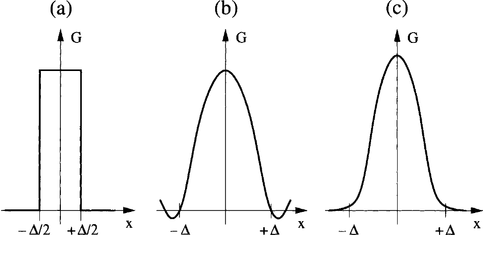
图7.3:物理空间中的LES滤波函数:tophat (a),cut-off (b),Gaussian (c)。图例:G——滤波函数;x——空间坐标;\(-\Delta/2\)、\(+\Delta/2\)——tophat滤波的支撑区间;\(-\Delta\)、\(+\Delta\)——滤波宽度标记。
7.3.2 Filtered Governing Equations 滤波控制方程[cfd-7-3-2]
为了去除小的湍流尺度,必须把由方程(7.76)和方程(7.77)定义的空间滤波作用于Navier-Stokes方程。滤波宽度\(\Delta\)和滤波函数都被视为自由参数。实际上,控制方程通常并不显式滤波,而是假定网格以及离散误差定义了滤波函数\(G\)。关于显式滤波的讨论见文献[116]、[117]。en
The spatial filtering, defined by Eq. (7.76) and Eq. (7.77), has to be applied to the Navier-Stokes equations in order to remove the small turbulent scales. The filter width \(\Delta\) as well as the filter function are considered as free parameters. In fact, the governing equations are usually not explicitly filtered. Instead, the grid as well as the discretisation errors are assumed to define the filter \(G\). For the discussion of explicit filtering see Refs. [116], [117].
由于处理方式不同,下文中我们将区分Navier-Stokes方程的可压缩形式(7.1)与不可压缩形式(7.6)。en
Because of the differing treatment, we shall distinguish in the following between compressible (7.1) and incompressible (7.6) formulation of the Navier-Stokes equations.
Incompressible Navier-Stokes Equations 不可压 Navier-Stokes 方程
对牛顿流体的不可压缩流动,滤波后的控制方程(7.6)取如下形式en
For an incompressible flow of a Newtonian fluid, the filtered governing equations (7.6) take the form
其中\(\nu\)表示运动黏度系数。方程(7.81)描述了承载能量的大尺度运动的时空演化。对流项的非线性导致出现所谓的亚网格尺度应力(subgrid-scale stress,SGS)张量en
where \(\nu\) denotes the kinematic viscosity coefficient. The equations (7.81) describe the temporal and spatial evolution of the large, energy-carrying scales of motion. The non-linearity of the convective term leads to the appearance of the so-called subgrid-scale stress (SGS) tensor
它描述不可解析尺度的影响。为了使方程封闭,必须对SGS张量建模(见小节7.3.3)。en
which describes the effects of the unresolved scales. The SGS tensor has to be modelled (see Subsection 7.3.3) in order to close the equations.
SGS张量可以分解为三个部分[118],即en
The SGS tensor can be decomposed into three parts [118], namely
各部分的物理含义如下:en
The individual parts have the following physical meaning:
为所谓的Leonard应力(Leonard stress)项,它代表产生小尺度湍流的大涡之间的相互作用。只有这一项可以由滤波速度场\(v_i\)显式求出。其次,交叉应力(cross-stress)项en
is the so-called Leonard stress term and represents the interactions between large-scale eddies which produce small-scale turbulence. This term only can be evaluated explicitly from the filtered velocity field \(v_i\). Further, the cross-stress term
描述大涡与小涡之间的相互作用。最后,en
describes interactions between large- and small-scale eddies. Finally,
为所谓的SGS雷诺应力(SGS Reynolds-stress)张量,它反映小尺度结构之间的相互作用。上述分解(7.83)如今已不再使用,主要原因是\(L_{ij}\)和\(C_{ij}\)在伽利略变换¹下不具有不变性。en
is the so-called SGS Reynolds-stress tensor. It reflects interactions between the small-scale structures. The above decomposition (7.83) is no longer used mainly because \(L_{ij}\) and \(C_{ij}\) are not invariant with respect to Galilean transformation¹.
¹原书脚注:Galilean invariance means that all frames of reference which are translating uniformly with respect to each other are equivalent.(伽利略不变性指的是,彼此做匀速平移的所有参考系都是等价的。)
Compressible Navier-Stokes Equations 可压缩 Navier-Stokes 方程
若要将LES应用于可压缩流动,就必须在对方程(7.1)做空间滤波的同时施加Favre平均(小节7.1.2)。否则,滤波后的Navier-Stokes方程将包含密度与速度、温度等其他变量的乘积。于是,式(7.1)中的速度分量、能量和温度按如下方式分解en
If LES is to be applied to compressible flows, we have to apply Favre averaging (Subsection 7.1.2) together with the spatial filtering to the Equations (7.1). Otherwise, the filtered Navier-Stokes equations would contain products between density and other variables like velocity or temperature. Thus, the velocity components, the energy and the temperature in Eq. (7.1) is decomposed as
空间中\(\vec{r}_0\)处的Favre滤波变量由下式给出en
The filtered variable at the location \(\vec{r}_0\) in space is given by
其中的各项为en
with the terms
以及en
and
在上述方程(7.89)-(7.90)中,\(e\)表示单位质量的内能,\(\tilde{S}_{ij}\)是Favre滤波应变率张量,\(\tau_{ij}^{SF} = \overline{\rho}\left(\widetilde{v_i v_j} - \tilde{v}_i\tilde{v}_j\right)\)表示Favre平均的亚网格尺度应力。此外,\(\mu\)、\(\mu_B\)和\(k\)分别表示分子黏度、体积黏度和热导率;而\(\tilde{\mu}\)、\(\tilde{\mu}_B\)和\(\tilde{k}\)是它们在滤波温度\(\tilde{T}\)下的对应取值。en
In the above equations (7.89)-(7.90), \(e\) denotes internal energy per unit mass, \(\tilde{S}_{ij}\) is the Favre-filtered strain-rate tensor, and \(\tau_{ij}^{SF} = \overline{\rho}\left(\widetilde{v_i v_j} - \tilde{v}_i\tilde{v}_j\right)\) represents the Favre-averaged subgrid-scale stress. Furthermore, \(\mu\), \(\mu_B\), and \(k\) stand for the molecular viscosity, the bulk viscosity, and for the thermal conductivity, respectively. Finally, \(\tilde{\mu}\), \(\tilde{\mu}_B\), and \(\tilde{k}\) are the corresponding values at the filtered temperature \(\tilde{T}\).
方程(7.89)的右端含有必须建模的项。在动量方程中,SGS应力\(\tau_{ij}^{SF}\)被近似,而第二项即\(\left(\overline{\sigma}_{ij} - \hat{\sigma}_{ij}\right)\)通常被忽略。在能量方程中,项\(\mathcal{A}\)可以通过SGS应力表达[119],项\(\mathcal{B}\)可以忽略,项\(\mathcal{C}\)、\(\mathcal{D}\)可按文献[120]所建议的方式建模。en
The right-hand side of Eq. (7.89) contains terms which have to be modelled. In the momentum equation, the SGS stresses \(\tau_{ij}^{SF}\) are approximated, but the second term, i.e., \(\left(\overline{\sigma}_{ij} - \hat{\sigma}_{ij}\right)\) is usually neglected. In the energy equation, term \(\mathcal{A}\) can be expressed through the SGS stresses [119], term \(\mathcal{B}\) can be neglected, and terms \(\mathcal{C}\), \(\mathcal{D}\) can be modelled as proposed in [120].
7.3.3 Subgrid-Scale Modelling 亚网格尺度建模[cfd-7-3-3]
亚网格尺度(subgrid-scale)模型的主要任务是模拟大尺度与亚网格尺度之间的能量传递。平均而言,能量从大尺度输运到小尺度(湍流串级过程)。因此,亚网格尺度模型必须提供充分的能量耗散手段。但在某些情形下,能量也会从小尺度流向大尺度——这一过程称为反向散射(backscatter)。因此模型也应当考虑这一效应。反向散射模型可参见例如[121]。en
The main task of a subgrid-scale model is to simulate energy transfer between the large and the subgrid scales. On the average, the energy is transported from the large scales to the small ones (turbulent cascade process). Therefore, a subgrid-scale model has to provide means of adequate energy dissipation. However, in some instances the energy also flows from small to large scales - a process called backscatter. Thus, the model should account for this effect as well. Backscatter models are discussed, e.g., in [121].
过去已提出多种亚网格尺度模型,研究至今仍在继续。这些模型可分为两大类。第一类是显式地建模SGS张量\(\tau_{ij}^S\)的方法,此时必要条件是空间离散格式引起的数值耗散必须远低于亚网格尺度耗散。大多数显式SGS模型基于涡黏性概念,下面将予以说明。此外,我们还将介绍构成所有亚网格尺度模型基础的Smagorinsky模型,并简要讨论所谓动力亚网格尺度(dynamic subgrid-scale)模型的基础。六种不同显式亚网格尺度模型的比较最近见于[122]。en
Various subgrid-scale models were proposed in the past and the research still continues. The models can be divided into two basic classes. The first one consists of approaches which model the SGS tensor \(\tau_{ij}^S\) explicitly. A necessary condition is then that the numerical dissipation caused by the spatial discretisation scheme must be much lower than the subgrid-scale dissipation. The majority of explicit SGS models is based on the eddy-viscosity concept, which is explained next. Furthermore, we shall present the Smagorinsky model, which forms the basis of all subgrid-scale models. We shall also briefly discuss the basics of the so-called dynamic subgrid-scale models. A comparison of six different explicit subgrid-scale models was presented recently in [122].
第二类亚网格尺度模型是通过对流通量的适当离散来隐式地模拟SGS应力(即略去\(\tau_{ij}^S\))的方法。这类模型称为单调积分大涡模拟(Monotonically Integrated LES,MILES)。该方法最早由Boris等[123]提出,近来由Grinstein和Fureby大力提倡[124]、[125]。此处的条件是数值耗散要正确地模拟亚网格尺度耗散。这并不容易做到,文献[126]和[127]的研究证明了这一点。尽管如此,MILES已在多种流动问题上取得了一定成功[128]-[134]。en
The second class of subgrid-scale models consists of approaches where the SGS stresses are modeled implicitly by an appropriate discretisation of the convective fluxes (thus \(\tau_{ij}^S\) is omitted). These models are referred to as Monotonically Integrated LES (MILES). The methodology was first presented by Boris et al. [123] and recently advocated by Grinstein and Fureby [124], [125]. The condition in this case is that the numerical dissipation correctly models the subgrid-scale dissipation. This is not quite easy to achieve, as the investigations in Ref. [126] and [127] prove. Nevertheless, MILES was applied with some success to a variety of flow problems [128]-[134].
Eddy-Viscosity Models 涡黏性模型
这些显式模型能够表现小尺度的全局耗散效应,但无法再现能量交换的局部细节。对不可压缩流动,涡黏性模型把SGS应力与大尺度应变率\(\overline{S}_{ij}\)联系起来如下en
These explicit models are able to represent the global dissipative effects of the small scales, but they cannot reproduce the local details of the energy exchange. In the case of incompressible flows, the eddy-viscosity models relate the SGS stresses to the large-scale strain-rate \(\overline{S}_{ij}\) as follows
应变率\(\overline{S}_{ij}\)由式(7.3)用滤波后的速度分量得到。为节省计算量,涡黏性\(\nu_T\)一般用代数关系式求值。SGS应力的各向同性部分(\(\tau_{kk}^S\))可以并入滤波压力[135]、单独建模[136]或忽略。en
The strain-rate \(\overline{S}_{ij}\) is obtained from Eq. (7.3) by using filtered velocity components. The eddy viscosity \(\nu_T\) is in general evaluated from algebraic relations in order to save numerical costs. The isotropic part of the SGS stresses (\(\tau_{kk}^S\)) can either be added to the filtered pressure [135], modelled [136] or neglected.
Smagorinsky SGS Model Smagorinsky SGS 模型
Smagorinsky模型[75]基于平衡假设,即小尺度把从大尺度接收到的能量全部、瞬时地耗散掉。该代数模型取如下形式en
The Smagorinsky model [75] is based on the equilibrium hypothesis which implies that the small scales dissipate entirely and instantaneously all the energy they receive from the large scales. The algebraic model assumes the form
其中\(|\overline{S}| = \left(2\overline{S}_{ij}\overline{S}_{ij}\right)^{1/2}\)为应变率张量的大小,\(C_s\)为Smagorinsky常数(Smagorinsky constant)。Lilly[137]求得的理论值为\(C_s \approx 0.18\)。但Smagorinsky常数依赖于流动类型,例如在剪切流中\(C_s\)须减小到约0.1。方程(7.93)中的滤波宽度\(\Delta\)通常取平均网格尺寸的两倍,即\(\Delta = 2\left(\Delta x_1\,\Delta x_2\,\Delta x_3\right)^{1/3}\)。en
where \(|\overline{S}| = \left(2\overline{S}_{ij}\overline{S}_{ij}\right)^{1/2}\) is the magnitude of the strain-rate tensor and \(C_s\) denotes the Smagorinsky constant. The theoretical value found by Lilly [137] is \(C_s \approx 0.18\). However, the Smagorinsky constant depends on the type of the flow. For example, in shear flows \(C_s\) has to be reduced to approximately 0.1. The filter width \(\Delta\) in Eq. (7.93) is usually chosen to be twice the average grid size, i.e., \(\Delta = 2\left(\Delta x_1\,\Delta x_2\,\Delta x_3\right)^{1/3}\).
为了体现近壁处小尺度增长的减弱,必须减小涡黏性\(\nu_T\)的取值。于是,Smagorinsky模型——方程(7.93)——按Van Driest阻尼修改为en
In order to account for the reduced growth of the small scales near walls, the value of the eddy viscosity \(\nu_T\) has to be reduced. Thus, the Smagorinsky model Eq. (7.93) is modified according to Van Driest damping as
其中\(y^{+}\)表示无量纲壁面距离(壁面距离的计算参见例如文献[39])。en
where \(y^{+}\) represents the dimensionless wall distance (for the computation of wall distances see, e.g., Ref. [39]).
Smagorinsky模型计算代价低、易于实现,但它有若干严重缺点:
- 在有平均剪切的层流区域中它耗散过强;
- 在壁面附近以及层流-湍流转捩处需要特殊处理;
- 参数\(C_s\)没有唯一定义;
- 没有模拟能量反向散射过程。
en
The Smagorinsky model is numerically cheap and easy to implement. However, it has several serious disadvantages:
- it is too dissipative in laminar regions with mean shear;
- it requires special provisions near walls and at laminar-turbulent transition;
- the parameter \(C_s\) is not uniquely defined;
- the process of energy backscatter is not modelled.
由于这些缺陷,人们提出了各种其他方法(参见例如[111])。下面这些动力模型非常流行。en
Because of these shortcomings, various other approaches were proposed (see, e.g., [111]). Very popular are the following dynamic models.
Dynamic SGS Models 动力 SGS 模型
动力SGS模型在计算方程(7.91)或(7.92)中的涡黏性\(\nu_T\)时,采用与Smagorinsky模型(方程(7.93))相同的关系式。区别在于:事先调整的Smagorinsky常数被一个在空间和时间中动态演化的参数所取代,即en
The dynamic SGS models employ the same relation as the Smagorinsky model (Eq. (7.93)) for the evaluation of the eddy viscosity \(\nu_T\) in Eq. (7.91) or (7.92). The difference is that the Smagorinsky constant (adjusted a priori) is replaced by a parameter, which evolves dynamically in space and in time. Hence,
参数\(C_d\)依据湍流最小尺度的能量含量来计算。为此,Germano等[138]提出采用第二个滤波——所谓的测试滤波(test filter)\(\hat{\Delta}\)。测试滤波的宽度必须大于作用于控制方程的滤波宽度\(\Delta\)(通常\(\hat{\Delta} = 2\Delta\))。把测试滤波作用于已滤波的方程,便得到所谓的亚测试尺度应力(subtest-scale stresses)\(\tau_{ij}^{ST}\)en
The parameter \(C_d\) is computed based on the energy content of the smallest scale of the turbulence. For this purpose, Germano et al. [138] proposed to employ a second filter - the so-called test filter \(\hat{\Delta}\). The width of the test filter has to be larger than that of the filter \(\Delta\) applied to the governing equations (usually \(\hat{\Delta} = 2\Delta\)). The application of the test filter to the filtered equations leads to the so-called subtest-scale stresses \(\tau_{ij}^{ST}\)
其中\(\hat{L}_{ij}\)表示与测试滤波相关的Leonard应力,它代表长度介于滤波宽度\(\Delta\)与测试滤波宽度\(\hat{\Delta}\)之间的尺度对雷诺应力的贡献。en
where \(\hat{L}_{ij}\) denotes the Leonard stresses associated with the test filter. It represents the contribution to the Reynolds stresses by the scales whose length is intermediate between the filter width \(\Delta\) and the test filter width \(\hat{\Delta}\).
其中en
with
记号\([\,]^{\wedge}\)表示方括号中的整个项都经过测试滤波。参数\(C_d\)可以利用Lilly的最小二乘极小化[140]从方程(7.98)导出,这给出en
The notation \([\,]^{\wedge}\) means that the whole term enclosed in the square brackets is test-filtered. The parameter \(C_d\) can be derived from Eq. (7.98) by using the least-squares minimisation of Lilly [140]. This leads to
改进的动力SGS模型由Ghosal等[141]、Carati等[142]、Piomelli和Liu[143]以及Held[90]等人提出。en
Improved dynamic SGS models were proposed, e.g., by Ghosal et al. [141], Carati et al. [142], Piomelli and Liu [143], and Held [90].
7.3.4 Wall Models 壁面模型[cfd-7-3-4]
对高雷诺数(\(Re > 10^6\))有壁流动做LES的计算代价对工程应用而言仍然过高,原因在于恰当解析壁面层需要过多的网格点(单元)。为了降低代价,可以通过指定外流速度与壁面应力之间的关联来对壁面层建模。这一做法与RANS模拟中使用壁面函数相当类似。其基本假设是近壁区与外区之间只有弱的相互作用,文献[144]和[145]的研究支持这一假设。en
The computational costs of LES of wall-bounded flows at high Reynolds numbers (\(Re > 10^6\)) are still too high for engineering purposes. The reason is the excessively large number of grid points (cells) required to resolve the wall layer appropriately. In order to reduce the costs, it is possible to model the wall layer by specifying a correlation between the velocity in the outer flow and the stress at the wall. This approach is quite similar to using wall functions in RANS simulations. The basic assumption is that there is only a weak interaction between the near-wall and the outer region, which is supported by the investigations in [144] and [145].
早期的壁面模型基于这样一种假设:壁面层的动力学是普适的,因而可以用广义壁面律来近似。这些模型基本上利用对数律(见[77]和[146]-[148])。Balaras等[149]最近提出了一种新的分区(zonal)方法。在两层模型中,滤波后的Navier-Stokes方程(7.81)一直求解到壁面上方第一个网格点;从该点到壁面之间,则在加密的嵌入网格上求解二维边界层方程。嵌入网格上的解随后用于给定壁面剪切应力,作为LES的边界条件。Balaras等[149]的分区方法允许把第一个点放在\(20 < y^{+} < 100\)的区域内,从而显著减小网格规模并缩短计算时间。该方法已成功应用于平面槽道、方形管道和旋转槽道中的湍流流动;后来又被用于分离流动的LES,结果令人鼓舞[150]-[153]。en
Earlier implementations of the wall models were based on the assumption that the dynamics of the wall layer are universal and hence they can be approximated by a generalised law-of-the-wall. Basically, the models utilised the logarithmic law (see [77] and [146]-[148]). Balaras et al. [149] proposed recently a new zonal approach. Within the two-layer model, the filtered Navier-Stokes equations (7.81) are solved up to the first grid point above the wall. From this point to the wall 2-D boundary layer equation are solved on a refined embedded grid. The solution on the embedded grid is then used to prescribe the wall shear stress as a boundary condition for the LES. The zonal approach of Balaras et al. [149] allows it to place the first point in a region \(20 < y^{+} < 100\), which leads to significantly reduced grid size and hence computational time. The methodology was applied with success to turbulent flows in a plane channel, square duct and rotating channel. Later on, it was also employed for the LES of separated flows with encouraging results [150]-[153].
7.3.5 Detached Eddy Simulation 脱体涡模拟[cfd-7-3-5]
尽管上述壁面模型有助于大幅减少网格点(单元)数量,但对于复杂的工程外形,LES仍然过于昂贵。为此,Spalart最近提出了另一种方法——所谓的脱体涡模拟(Detached Eddy Simulation,DES),其目标是高雷诺数大范围分离流动的模拟[154]、[155]。该方法可以说是RANS与LES的混合体:其思想是在强拉伸网格上配合RANS湍流模型(大多是Spalart-Allmaras模型,见小节7.2.1,或Menter的SST模型,见小节7.2.3)来解析附着边界层,而在壁面区之外配合各向同性网格使用LES来捕捉脱体的三维涡。这样,DES试图在一个统一框架内结合两种方法的长处。en
Even though the above wall models help to reduce the number of grid points (cells) considerably, LES still remains too costly for complex engineering configurations. For this reason, Spalart recently suggested another approach, the so-called Detached Eddy Simulation (DES), which is aimed at the simulation of high Reynolds-number massively separated flows [154], [155]. The methodology represents a hybrid between the RANS and LES. The idea is to employ highly stretched grids together with a RANS turbulence model (mostly the Spalart-Allmaras model from Subsection 7.2.1 or Menter's SST model from Subsection 7.2.3) to resolve the attached boundary layer(s), and to use LES outside the wall region together with an isotropic grid to capture the detached 3-D eddies. Thus, DES tries to combine the strengths of both methods in a single framework.
该长度尺度取决于控制体的最大尺寸,即\(\Delta = \max(\Delta x, \Delta y, \Delta z)\)。常数\(C_{DES}\)在一定程度上依赖于流动类型:对均匀湍流,发现\(C_{DES} = 0.65\)最优[156];而对跨声速和超声速射流,则建议取\(C_{DES} = 0.1\)[157]。方程(7.102)中长度尺度\(l\)的定义保证了:在边界层内,那里\(d < C_{DES}\Delta\)、因而\(l = d\),恢复出原始的RANS模型;而在边界层之外\(l = C_{DES}\Delta\),Spalart-Allmaras模型则充当LES的单方程SGS模型(对照方程(7.91)和式(7.24))。在时间方向积分控制方程时,全局时间步长必须调整到能够解析脱体涡的时间尺度。这通常意味着时间步长会远远超出显式格式在边界层区域的稳定裕度。因此更高效的做法是采用时间精确的隐式格式,例如6.3节所述的双时间步进方法。关于DES方法的更多细节和模拟实例可参见上述文献或[158]-[161]。en
The length scale is dependent on the largest dimension of the control volume, i.e., \(\Delta = \max(\Delta x, \Delta y, \Delta z)\). The constant \(C_{DES}\) depends to some extent on the type of the flow. For a homogeneous turbulence, the value \(C_{DES} = 0.65\) was found optimal [156]. On the other hand, \(C_{DES} = 0.1\) was recommended for transonic and supersonic jets [157]. The definition of the length scale \(l\) in Eq. (7.102) makes sure that within the boundary layer, where \(d < C_{DES}\Delta\) and hence \(l = d\), the original RANS model is recovered. On the other hand, outside the boundary layer \(l = C_{DES}\Delta\) and the Spalart-Allmaras model serves as a one-equation SGS model for the LES (cf. Eq. (7.91) and (7.24)). When integrating the governing equations in time, the global time step has to be adjusted such as to resolve the time scales of the detached eddies. This usually means that the time step would by far exceed the stability margin of an explicit scheme for the boundary layer region. It is therefore more efficient to employ a time-accurate implicit scheme, such as the dual time-stepping approach described in Section 6.3. More details regarding the DES methodology and examples of simulations can be found in the above references or in [158]-[161].