7.1 Basic Equations of Turbulence 湍流的基本方程[cfd-7-1]
首先,让我们把控制方程(2.19)改写成微分形式(见附录A.1),因为湍流建模文献中经常使用这种形式;此外,它还使记号紧凑而清晰。不过,我们也会给出湍流方程积分形式的例子。en
First of all, let us rewrite the governing equations (2.19) in differential form (see Appendix A.1), since this is used very often in literature on turbulence modelling. Furthermore, it allows for a compact and clear notation. However, we will also provide examples of turbulence equations in integral form.
对于可压缩Newton流体,在无源项的情形下,Navier-Stokes方程按坐标不变量形式写为en
In the case of a compressible Newtonian fluid, the Navier-Stokes equations read in the absence of source terms in coordinate invariant formulation as
在上述方程(7.1)中,\(v_i\)表示一个速度分量(\(\vec{v}=\left[v_1,v_2,v_3\right]^T\)),\(x_i\)代表一个坐标方向。关于紧凑张量记号的说明见附录A.13。en
In above Eq. (7.1), \(v_i\) denotes a velocity component (\(\vec{v}=\left[v_1,v_2,v_3\right]^T\)), and \(x_i\) stands for a coordinate direction, respectively. An explanation of the compact tensor notation can be found in Appendix A.13.
其中利用了Stokes假设(式(2.17))。在直角坐标系下,式(7.2)与式(2.15)等价。式(7.2)中的第二项,即\(\partial v_k/\partial x_k\),对应于速度的散度,在不可压缩流动中为零。应变率张量(strain-rate tensor)的分量由下式给出en
where we utilised the Stokes's hypothesis (Eq. (2.17)). In Cartesian coordinates, Eq. (7.2) is equivalent to Eq. (2.15). The second term in Eq. (7.2), i.e., \(\partial v_k/\partial x_k\), which corresponds to the divergence of the velocity, disappears for incompressible flows. The components of the strain-rate tensor are given by
与此同时,让我们再定义旋转率张量(rotation-rate tensor,即速度梯度张量的反对称部分),其分量为en
In this connection, let us also define the rotation-rate tensor (antisymmetric part of the velocity gradient tensor) with the following components
它们在直角坐标系中分别对应于式(2.6)和式(2.12)。en
which correspond in Cartesian coordinate system to Eq. (2.6) and Eq. (2.12), respectively.
其中\(\nu=\mu/\rho\)为运动黏性系数,\(\nabla^2\)表示拉普拉斯算子。在没有浮力效应时,温度\(T\)的方程与质量守恒方程和动量方程解耦。en
with \(\nu=\mu/\rho\) being the kinematic viscosity coefficient and \(\nabla^2\) denoting the Laplace operator. In the absence of buoyancy effects, the equation for the temperature \(T\) becomes decoupled from the mass conservation and momentum equations.
7.1.1 Reynolds Averaging 雷诺平均[cfd-7-1-1]
对湍流进行近似处理的第一种方法由Reynolds于1895年提出。该方法基于把流动变量分解为平均值与脉动值两部分。随后求解控制方程(7.1)的平均值——平均值对工程应用最有意义。这样,首先考虑不可压缩流动,方程(7.1)中的速度分量和压力用下式替代[13]en
The first approach for the approximate treatment of turbulent flows was presented by Reynolds in 1895. The methodology is based on the decomposition of the flow variables into a mean and a fluctuating part. The governing equations (7.1) are then solved for the mean values, which are the most interesting for engineering applications. Thus, considering first incompressible flows, the velocity components and the pressure in Eq. (7.1) are substituted by [13]
其中平均值用上划线表示,湍流脉动用撇号表示。平均值通过平均过程求得。雷诺平均(Reynolds averaging)有三种不同的形式:en
where the mean value is denoted by an overbar and the turbulent fluctuations by a prime. The mean values are obtained by an averaging procedure. There are three different forms of the Reynolds averaging:
1. 时间平均(time averaging)——适用于定常湍流(统计定常湍流)en
1. Time averaging -- appropriate for stationary turbulence (statistically steady turbulence)
其结果是,平均值\(\bar{v}_i\)不随时间变化,而只随空间变化。情形如图7.2所示。实践中,\(T\to\infty\)意味着时间间隔\(T\)应远大于湍流脉动的典型时间尺度。en
As a consequence, the mean value \(\bar{v}_i\) does not vary in time, but only in space. The situation is sketched in Fig. 7.2. In practice, \(T\to\infty\) means that the time interval \(T\) should be large as compared to the typical time-scale of the turbulent fluctuations.
2. 空间平均(spatial averaging)——适用于均匀湍流en
2. Spatial averaging -- appropriate for homogeneous turbulence
其中\(\Omega\)为控制体。此时\(\bar{v}_i\)在空间上均匀,但允许随时间变化。en
with \(\Omega\) being a control volume. In this case, \(\bar{v}_i\) is uniform in space, but it is allowed to vary in time.
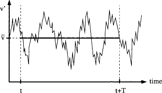
图7.2:雷诺平均——湍流速度脉动\(v'\)与统计平均值\(\bar{v}\)的示意图。
3. 系综平均(ensemble averaging)——适用于一般湍流en
3. Ensemble averaging -- appropriate for general turbulence
这里,平均值\(\bar{v}_i\)仍然是时间和空间坐标的函数。en
Here, the mean value \(\bar{v}_i\) still remains a function of time and of space coordinates.
对所有这三种方法,脉动部分的平均值都为零,即\(\overline{v'_i}=0\)。然而,容易看出\(\overline{v'_iv'_i}\neq 0\)。若两个湍流速度分量相关,则对\(\overline{v'_iv'_j}\)同样如此。en
For all three approaches, the average of the fluctuating part is zero, i.e., \(\overline{v'_i}=0\). However, it can be easily seen that \(\overline{v'_iv'_i}\neq 0\). The same is true for \(\overline{v'_iv'_j}\), if both turbulent velocity components are correlated.
当湍流既是定常的又是均匀的时候,三种平均形式彼此等价。这称为各态历经假设(ergodic hypothesis)。en
In cases where the turbulent flow is both stationary and homogeneous, all three averaging forms are equivalent. This is called the ergodic hypothesis.
7.1.2 Favre (Mass) Averaging Favre(质量)平均[cfd-7-1-2]
在密度不为常数的情形下,对方程(7.1)中的某些量,宜采用密度(质量)加权即Favre分解[14]、[15]来代替雷诺平均。否则,由于出现涉及密度脉动的额外关联,平均后的控制方程会变得复杂得多。最方便的做法是:对密度和压力采用雷诺平均,对速度、内能、焓和温度等其他变量采用Favre平均。Favre平均量(例如速度分量)由如下关系求得[14]、[15]en
In cases where the density is not constant, it is advisable to apply the density (mass) weighted or Favre decomposition [14], [15] to certain quantities in Eq. (7.1) instead of Reynolds averaging. Otherwise, the averaged governing equations would become considerably more complicated due to additional correlations involving density fluctuations. The most convenient way is to employ Reynolds averaging for density and pressure, and Favre averaging for other variables such as velocity, internal energy, enthalpy and temperature. Favre averaged quantities, for example the velocity components, are obtained from the relation [14], [15]
其中\(\bar{\rho}\)表示雷诺平均密度。于是,Favre分解写为en
where \(\bar{\rho}\) denotes the Reynolds-averaged density. Hence, the Favre decomposition reads
其中\(\tilde{v}_i\)表示平均值,\(v''_i\)表示速度\(v_i\)的脉动部分。同样,脉动部分的平均值为零,即\(\widetilde{v''_i}=0\)。此外,若两个脉动量相关,则其乘积的平均值不为零。例如,\(\widetilde{v''_iv''_i}\neq 0\),并且一般地\(\widetilde{v''_iv''_j}\neq 0\)。en
where \(\tilde{v}_i\) represents the mean value and \(v''_i\) the fluctuating part of the velocity \(v_i\). Again, the average of the fluctuating part is zero, i.e., \(\widetilde{v''_i}=0\). Furthermore, the average of the product of two fluctuating quantities is not zero, if the quantities are correlated. Hence, for example, \(\widetilde{v''_iv''_i}\neq 0\) and in general \(\widetilde{v''_iv''_j}\neq 0\).
对于Favre平均与雷诺平均的混合使用,可以导出如下关系en
The following relationships can be derived for a mix between Favre and Reynolds averaging
这些关系将在后面的小节中用到。en
These relations will be utilised in later subsections.
7.1.3 Reynolds-Averaged Navier-Stokes Equations 雷诺平均Navier-Stokes方程[cfd-7-1-3]
雷诺应力张量在三维情形下由九个分量组成en
The Reynolds-stress tensor consists in 3D of the nine components
不过,由于关联中的\(v'_i\)与\(v'_j\)可以互换,雷诺应力张量只包含六个独立分量。各法向应力之和除以密度即定义为湍动能(turbulent kinetic energy),即en
However, since \(v'_i\) and \(v'_j\) in the correlations can be interchanged, the Reynolds-stress tensor contains only six independent components. The sum of the normal stresses divided by density defines the turbulent kinetic energy, i.e.,
如我们所见,基于雷诺平均Navier-Stokes方程的湍流建模,其根本问题在于找出六个附加关系式,以使方程(7.14)封闭。我们将在7.1.5–7.1.7小节中介绍基本方法。en
As we can see, the fundamental problem of turbulence modelling based on the Reynolds-averaged Navier-Stokes equations is to find six additional relations in order to close the equations (7.14). We shall introduce the basic methodologies in the Subsections 7.1.5--7.1.7.
7.1.4 Favre- and Reynolds-Averaged Navier-Stokes Equations Favre平均与雷诺平均Navier-Stokes方程[cfd-7-1-4]
在湍流建模中,通常假设Morkovin假设[16]成立。该假设指出:若\(\rho'\ll\bar{\rho}\),边界层的湍流结构不会受到密度脉动的显著影响。对于壁面约束流动,直到马赫数约为5这一结论一般都成立。然而,对于高超声速流动或可压缩自由剪切层,则必须计及密度脉动。对于有燃烧或有显著传热的流动,情况也是如此。en
In turbulence modelling, it is quite common to assume that Morkovin's hypothesis [16] is valid. It states that the turbulent structure of a boundary layer is not notably influenced by density fluctuations if \(\rho'\ll\bar{\rho}\). This is generally true for wall-bounded flows up to a Mach number of about five. However, in the case of hypersonic flows or for compressible free shear layers, density fluctuations have to be taken into account. The same holds also for flows with combustion or with significant heat transfer.
这就是Favre平均与雷诺平均Navier-Stokes方程。与雷诺平均类似,动量(和能量)方程中的黏性应力张量要再加上Favre平均雷诺应力张量,即en
These are the Favre- and Reynolds-Averaged Navier-Stokes equations. Similarly to the Reynolds averaging, the viscous stress tensor in the momentum (and energy) equation is extended by the Favre-averaged Reynolds-stress tensor, i.e.,
如果采用Favre平均湍动能的定义,即en
If we employ the definition of the Favre-averaged turbulent kinetic energy, i.e.,
总焓定义为en
The total enthalpy is defined as
Favre平均与雷诺平均Navier-Stokes方程(7.19)的各个部分具有如下物理意义[17]:
- \(\dfrac{\partial}{\partial x_j}\left(k\dfrac{\partial\tilde{T}}{\partial x_j}\right)\)——热的分子扩散
- \(\dfrac{\partial}{\partial x_j}\left(\bar{\rho}\widetilde{v''_jh''}\right)\)——热的湍流输运
- \(\dfrac{\partial}{\partial x_j}\left(\widetilde{\tau_{ij}v''_i}\right)\)——\(\tilde{K}\)的分子扩散
- \(\dfrac{\partial}{\partial x_j}\left(\bar{\rho}\widetilde{v''_jK}\right)\)——\(\tilde{K}\)的湍流输运
- \(\dfrac{\partial}{\partial x_j}\left(\tilde{v}_i\bar{\tau}_{ij}\right)\)——分子应力做的功
- \(\dfrac{\partial}{\partial x_j}\left(\tilde{v}_i\tau^F_{ij}\right)\)——Favre平均雷诺应力做的功
en
The individual parts of the Favre- and Reynolds-averaged Navier-Stokes equations (7.19) have the following physical meaning [17]:
- \(\dfrac{\partial}{\partial x_j}\left(k\dfrac{\partial\tilde{T}}{\partial x_j}\right)\) - molecular diffusion of heat
- \(\dfrac{\partial}{\partial x_j}\left(\bar{\rho}\widetilde{v''_jh''}\right)\) - turbulent transport of heat
- \(\dfrac{\partial}{\partial x_j}\left(\widetilde{\tau_{ij}v''_i}\right)\) - molecular diffusion of \(\tilde{K}\)
- \(\dfrac{\partial}{\partial x_j}\left(\bar{\rho}\widetilde{v''_jK}\right)\) - turbulent transport of \(\tilde{K}\)
- \(\dfrac{\partial}{\partial x_j}\left(\tilde{v}_i\bar{\tau}_{ij}\right)\) - work done by the molecular stresses
- \(\dfrac{\partial}{\partial x_j}\left(\tilde{v}_i\tau^F_{ij}\right)\) - work done by the Favre-averaged Reynolds stresses
\(\tilde{K}\)的分子扩散和湍流输运在很多时候都可以忽略。对于跨声速和超声速流动,这是有效的近似。为使Favre平均与雷诺平均方程(7.19)封闭,还必须提供Favre平均雷诺应力张量(式(7.20))的六个分量以及湍流热通量向量的三个分量。我们将在后面几个小节中讨论这三种基本方法。en
The molecular diffusion and turbulent transport of \(\tilde{K}\) are very often neglected. This is a valid approximation for transonic and supersonic flows. In order to close the Favre- and Reynolds-averaged equations (7.19), we also have to supply six components of the Favre-averaged Reynolds-stress tensor (Eq. (7.20)) and three components of the turbulent heat-flux vector. We shall discuss the three basic approaches in the next subsections.
7.1.5 Eddy-Viscosity Hypothesis 涡黏性假设[cfd-7-1-5]
湍流建模领域最重要的贡献之一由Boussinesq于1877年作出[11]、[12]。他的想法基于如下观察:湍流中的动量输运由大而高能的湍流涡所引起的混合主导。Boussinesq假设湍流剪应力像层流中那样线性地依赖于平均应变率,其比例系数就是涡黏性(eddy viscosity)。对于雷诺平均不可压缩流动(式(7.14)),Boussinesq假设可以写为en
One of the most significant contributions to turbulence modelling was presented in 1877 by Boussinesq [11], [12]. His idea is based on the observation that the momentum transfer in a turbulent flow is dominated by the mixing caused by large energetic turbulent eddies. The Boussinesq hypothesis assumes that the turbulent shear stress depends linearly on the mean rate of strain, as in a laminar flow. The proportionality factor is the eddy viscosity. The Boussinesq hypothesis for Reynolds averaged incompressible flow (Eq. (7.14)) can be written as
其中\(\overline{S}_{ij}\)表示雷诺平均应变率张量(式(7.3),另见式(7.16)),\(K\)为湍动能(\(K=(1/2)\overline{v'_iv'_i}\)),\(\mu_T\)代表涡黏性。与分子黏性\(\mu\)不同,涡黏性\(\mu_T\)不是流体的物理特性,而是局部流动条件的函数。此外,\(\mu_T\)还受到流动历史效应的强烈影响。en
where \(\overline{S}_{ij}\) denotes the Reynolds-averaged strain-rate tensor (Eq. (7.3), cf. also Eq. (7.16)), \(K\) is the turbulent kinetic energy (\(K=(1/2)\overline{v'_iv'_i}\)), and \(\mu_T\) stands for the eddy viscosity. Unlike the molecular viscosity \(\mu\), the eddy viscosity \(\mu_T\) represents no physical characteristic of the fluid, but it is a function of the local flow conditions. Additionally, \(\mu_T\) is also strongly affected by flow history effects.
其中\(\tilde{S}_{ij}\)和\(\tilde{K}\)分别为Favre平均应变率和Favre平均湍动能。注意它与式(7.2)的相似性。式(7.24)和(7.25)中的\((2/3)\rho K\delta_{ij}\)项是为了得到\(\tau^R_{ij}\)或\(\tau^F_{ij}\)的正确迹(trace)所必需的。这意味着,我们必须有en
where \(\tilde{S}_{ij}\) and \(\tilde{K}\) are the Favre-averaged strain rate and turbulent kinetic energy, respectively. Note the similarity to Eq. (7.2). The term \((2/3)\rho K\delta_{ij}\) in Eqs. (7.24) and (7.25) is required in order to obtain the proper trace of \(\tau^R_{ij}\) or \(\tau^F_{ij}\). This means that we must have
即在\(\overline{S}_{ii}=0\)(连续方程)或\(\tilde{S}_{ii}=0\)的情形下,以满足湍动能的关系式(7.18)或(7.21)。然而,\((2/3)\rho K\delta_{ij}\)这一项常常被忽略,特别是在与较简单的湍流模型(如代数模型)联用时。en
in the case of \(\overline{S}_{ii}=0\) (continuity equation) or \(\tilde{S}_{ii}=0\), in order to fulfil the relations Eq. (7.18) or (7.21) for the turbulent kinetic energy. However, the term \((2/3)\rho K\delta_{ij}\) is often neglected, particularly in connection with simpler turbulence models (like algebraic ones).
对湍流热通量向量建模时常用的近似基于经典的Reynolds比拟[18]。于是,我们可以写en
The approximation, which is commonly used for the modelling of the turbulent heat-flux vector, is based on the classical Reynolds analogy [18]. Hence, we may write
其中湍流热导率系数(turbulent thermal conductivity coefficient)\(k_T\)定义为en
with the turbulent thermal conductivity coefficient \(k_T\) being defined as
在方程(7.27)中,\(c_p\)表示定压比热系数,\(Pr_T\)为湍流Prandtl数。一般假设湍流Prandtl数在整个流场中为常数(对空气\(Pr_T=0.9\))。en
In Equation (7.27), \(c_p\) denotes the specific heat coefficient at constant pressure and \(Pr_T\) is the turbulent Prandtl number. The turbulent Prandtl number is in general assumed to be constant over the flow field (\(Pr_T=0.9\) for air).
把涡黏性方法应用于控制方程(2.19)或方程(7.1)的雷诺(及Favre)平均形式时,黏性应力张量式(2.15)或式(7.2)中的动力黏性系数\(\mu\)被简单地替换为层流分量与湍流分量之和,即en
By applying the eddy-viscosity approach to the Reynolds- (and Favre-) averaged form of the governing equations (2.19) or Eq. (7.1), the dynamic viscosity coefficient \(\mu\) in the viscous stress tensor Eq. (2.15) or Eq. (7.2) is simply replaced by the sum of a laminar and a turbulent component, i.e.,
至少从工程的角度看,Boussinesq的涡黏性概念非常有吸引力,因为它“只”需要确定\(\mu_T\)(式(7.24)或(7.25)中\((2/3)\rho K\delta_{ij}\)项所需的湍动能\(K\),或者作为湍流模型的副产物得到,或者干脆略去)。一旦知道了涡黏性\(\mu_T\),通过引入平均流动变量并把\(\mu_T\)加到层流黏性上,我们就能容易地把Navier-Stokes方程(2.19)或(7.1)扩展用于湍流模拟。因此,Boussinesq方法成为了大量一阶湍流封闭的基础。然而,对某些应用而言,Boussinesq假设不再成立(例如见[17]第214页或[19]第111页):
- 平均应变率发生突然变化的流动;
- 具有显著流线曲率的流动;
- 具有旋转和分层的流动;
- 管道和透平机械中的二次流;
- 边界层分离与再附的流动。
en
The eddy-viscosity concept of Boussinesq is, at least from the engineering point of view, very attractive since it requires ``only'' the determination of \(\mu_T\) (the turbulent kinetic energy \(K\) needed for the term \((2/3)\rho K\delta_{ij}\) in Eq. (7.24) or (7.25) is either obtained as a by-product of the turbulence model or is simply omitted). Once we know the eddy viscosity \(\mu_T\), we can easily extend the Navier-Stokes equations (2.19) or (7.1) to the simulation of turbulent flows by introducing averaged flow variables and by adding \(\mu_T\) to the laminar viscosity. Therefore, Boussinesq's approach became the basis for a large variety of first-order turbulence closures. However, there are applications for which the Boussinesq hypothesis is no longer valid (see, e.g., [17] p. 214 or [19] p. 111):
- flows with sudden change of mean strain rate,
- flows with significant streamline curvature,
- flows with rotation and stratification,
- secondary flows in ducts and in turbomachinery,
- flows with boundary layer separation and reattachment.
涡黏性方法的局限源于把湍流与平均应变场视为处于平衡状态的假设,以及其结果与系统旋转无关的假定。通过在湍流模型中加入适当的修正项,结果可以明显改善[20]、[21]。采用下面要介绍的非线性涡黏性模型,可以进一步提高预测精度。en
The limitations of the eddy-viscosity approach are caused by the assumption of equilibrium between the turbulence and the mean strain field, as well as by the independence on system rotation. The results can be notably improved by using appropriate correction terms in the turbulence models [20], [21]. Further increased accuracy of predictions can be achieved through the application of non-linear eddy-viscosity models which are described next.
7.1.6 Non-Linear Eddy Viscosity 非线性涡黏性[cfd-7-1-6]
为了消除湍流与平均应变率之间平衡假设所强加的限制,Lumley[22]、[23]提议用应变张量与旋转张量的高阶乘积来扩展线性的Boussinesq方法。这可以视为一种Taylor级数展开。沿着Lumley的思路,人们提出了众多非线性涡黏性模型,例如文献[24]–[29]。en
In order to remove the restrictions imposed by the assumption of equilibrium between the turbulence and the mean strain rate, Lumley [22], [23] proposed to extend the linear Boussinesq approach by higher-order products of strain and rotation tensors. This can viewed as a Taylor series expansion. Following the idea of Lumley, numerous non-linear eddy-viscosity models were proposed, see, for example, Refs. [24]--[29].
下面我们介绍由Shih等人[25]提出的一种较新的方法。它在一般涡黏性表述中包含直至三阶的项,特别适合于旋转流(swirling flows)。正如文献[19]第194页所指出的,三次项对高精度至关重要。雷诺应力\(\tau^R_{ij}\)可以表示为[25]、[30](对照式(7.24))en
In the following, we shall present one recent approach proposed by Shih et al. [25]. It includes up to third-order terms in the general eddy-viscosity formulation and is particularly suited to swirling flows. As already pointed out in [19], p. 194, cubic terms are essential for high accuracy. The Reynolds stresses \(\tau^R_{ij}\) can be expressed as [25], [30] (cf. Eq. (7.24))
湍动能\(K\)和耗散率(dissipation rate)\(\varepsilon\)的值由低雷诺数\(K\)-\(\varepsilon\)湍流模型给出(参见7.2.2小节)。式(7.30)中的系数\(C_1\)至\(C_5\)见文献[25]、[30]。en
The values of the turbulent kinetic energy \(K\) and the dissipation rate \(\varepsilon\) are obtained from low-Reynolds \(K\)-\(\varepsilon\) turbulence model (cf. Subsection 7.2.2). The factors \(C_1\) to \(C_5\) in Eq. (7.30) are provided in Refs. [25], [30].
与线性涡黏性方法相比,非线性模型的计算代价只略微增大,但对复杂湍流的预测能力却有显著提高。en
In comparison to the linear eddy-viscosity approach, the non-linear models are computationally only slightly more expensive, but they offer a substantially improved prediction capabilities for complex turbulent flows.
7.1.7 Reynolds-Stress Transport Equation 雷诺应力输运方程[cfd-7-1-7]
通过取时间平均(二阶矩),可以为雷诺应力导出精确方程en
It is possible to derive exact equations for the Reynolds stresses by taking the time average (second-order moment)
其中\(\mathcal{N}(v_i)\)表示Navier-Stokes算子,即en
where \(\mathcal{N}(v_i)\) denotes the Navier-Stokes operator, i.e.,
它适用于不可压缩流动。可压缩流动的表述见文献[17]第179页,或[32]、[33]。方程(7.34)中,湍动能的生成项\(P_{ij}\)、压力—应变项\(\Pi_{ij}\)、耗散率项\(\varepsilon_{ij}\)以及三阶扩散项\(C_{ijk}\)定义为en
for incompressible flow. The formulation for compressible flows can be found in Ref. [17], p. 179, or in [32], [33]. The production of the turbulent kinetic energy \(P_{ij}\), the pressure-strain term \(\Pi_{ij}\), the dissipation-rate term \(\varepsilon_{ij}\), and the third-order diffusion term \(C_{ijk}\) in Eq. (7.34) are defined as
在方程(7.35)中,\(S'_{ij}\)表示应变率张量的脉动部分。\(C_{ijk}\)的第一部分(三重速度项)表示由脉动对流驱动的输运,另外两部分则分别是压力输运项(压力—速度关联)。en
In Eq. (7.35), \(S'_{ij}\) denotes the fluctuating part of the strain-rate tensor. The first part of \(C_{ijk}\), the triple velocity term, represents transport driven by fluctuating convection, the two other parts are the pressure transport terms (pressure-velocity correlations), respectively.
如我们所见,精确的雷诺应力方程包含新的未知高阶关联(例如\(\overline{v'_iv'_jv'_k}\))。因此,方程(7.34)只能借助经验模型来封闭。这是由Navier-Stokes方程的非线性本质造成的。二阶封闭——雷诺应力模型——为求解方程(7.34)提供了必要的框架。实施的例子可参见文献[34]–[36]。en
As we can see, the exact Reynolds-stress equation contains new unknown higher-order correlations (e.g., \(\overline{v'_iv'_jv'_k}\)). Therefore, Equation (7.34) can be closed only by using empirical models. This is caused by the non-linear nature of the Navier-Stokes equations. The second-order closures -- the Reynolds-stress models -- provide the necessary framework for solving Eq. (7.34). Examples of implementations can be found, e.g., in Refs. [34]--[36].