chapter. Governing Equations 第2章 控制方程[cfd-0003]
2.1 The Flow and its Mathematical Description 流动及其数学描述[cfd-2-1]
在开始推导描述流体行为的基本方程之前,先澄清“流体动力学(fluid dynamics)”这一术语的含义可能会更方便。实际上,它研究的是大量单个粒子之间的相互作用运动,在这里这些粒子就是分子或原子。这意味着,我们假定流体的密度足够高,以致可以把它近似为连续介质(continuum)。也就是说,即使是微分意义下无限小的流体微元,也仍然包含足够多的粒子,从而可以为其指定平均速度和平均动能。这样,我们就能够在流体的每一点上定义速度、压力、温度、密度以及其他重要物理量。en
Before we begin with the derivation of the basic equations describing the behaviour of the fluid, it may be convenient to clarify what the term 'fluid dynamics' stands for. It is, in fact, the investigation of the interactive motion of a large number of individual particles. These are in our case molecules or atoms. That means, we assume the density of the fluid is high enough, so that it can be approximated as a continuum. It implies that even an infinitesimally small (in the sense of differential calculus) element of the fluid still contains a sufficient number of particles, for which we can specify mean velocity and mean kinetic energy. In this way, we are able to define velocity, pressure, temperature, density and other important quantities at each point of the fluid.
流体动力学基本方程的推导基于这样一个事实:流体的动力学行为由以下守恒定律(conservation laws)决定,即:
- 质量守恒;
- 动量守恒;
- 能量守恒。
en
The derivation of the principal equations of fluid dynamics is based on the fact that the dynamical behaviour of a fluid is determined by the following conservation laws, namely:
- the conservation of mass,
- the conservation of momentum, and
- the conservation of energy.
某一流动量的守恒,意味着它在任意体积内部的总变化,可以表示为以下几方面的净效应:越过边界被输运的该量、体积内部可能存在的内力和源,以及作用在该体积上的外力。越过边界的该量之数量称为通量(flux)。通量一般可以分解为两个不同的部分:一个源于对流输运,另一个源于静止流体中存在的分子运动。后一部分具有扩散性质——它与所考虑物理量的梯度成正比,因此在均匀分布时为零。en
The conservation of a certain flow quantity means that its total variation inside an arbitrary volume can be expressed as the net effect of the amount of the quantity being transported across the boundary, of any internal forces and sources, and of external forces acting on the volume. The amount of the quantity crossing the boundary is called flux. The flux can be in general decomposed into two different parts: one due to the convective transport and the other one due to the molecular motion present in the fluid at rest. This second contribution is of a diffusive nature - it is proportional to the gradient of the quantity considered, and hence it will vanish for a homogeneous distribution.
对守恒定律的讨论很自然地引导我们产生这样一个想法:把流场划分成许多体积,并集中研究流体在其中某一个有限区域内的行为。为此,我们定义所谓的有限控制体(finite control volume),并试图对其物理性质建立数学描述。en
The discussion of the conservation laws leads us quite naturally to the idea of dividing the flow field into a number of volumes and to concentrate on the modelling of the behaviour of the fluid in one such finite region. For this purpose, we define the so-called finite control volume and try to develop a mathematical description of its physical properties.
Finite control volume 有限控制体
考察图2.1中以流线表示的一个一般流场。流场中由封闭曲面\(\partial\Omega\)所包围、固定在空间中的一个任意有限区域,定义了控制体\(\Omega\)。我们还引入面元\(dS\)及其相应的、指向外侧的单位法向量\(\vec{n}\)。en
Consider a general flow field as represented by streamlines in Fig. 2.1. An arbitrary finite region of the flow, bounded by the closed surface \(\partial\Omega\) and fixed in space, defines the control volume \(\Omega\). We also introduce a surface element \(dS\) and its associated, outward pointing unit normal vector \(\vec{n}\).
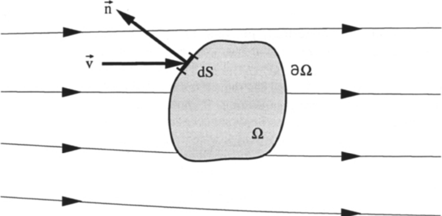
图2.1:有限控制体的定义(固定于空间中)。图例:流线;\(\Omega\)——控制体;\(\partial\Omega\)——控制体边界(封闭曲面);\(dS\)——面元;\(\vec{n}\)——外指单位法向量;\(\vec{v}\)——流动速度。
将守恒定律应用于单位体积上某个示例标量\(U\),则它在\(\Omega\)内随时间的变化,即en
The conservation law applied to an exemplary scalar quantity per unit volume \(U\) says that its variation in time within \(\Omega\), i.e.,
等于下列各项贡献之和:由对流通量(convective flux)引起的贡献——即以速度\(\vec{v}\)通过边界进入控制体的物理量\(U\)的数量en
is equal to the sum of the contributions due to the convective flux - amount of the quantity \(U\) entering the control volume through the boundary with the velocity \(\vec{v}\)
再加上由扩散通量(diffusive flux)引起的贡献——它由广义的Fick梯度定律表示en
further due to the diffusive flux - expressed by the generalised Fick's gradient law
其中\(\kappa\)为热扩散率系数(thermal diffusivity coefficient);最后还有体积源和面源\(Q_V\)、\(\vec{Q}_S\)的贡献,即en
where \(\kappa\) is the thermal diffusivity coefficient, and finally due to the volume as well as surface sources, \(Q_V\), \(\vec{Q}_S\), i.e.,
把上述各项贡献相加,便得到标量\(U\)的守恒定律的如下一般形式en
After summing up the above contributions, we obtain the following general form of the conservation law for the scalar quantity \(U\)
其中\(U^{*}\)表示单位质量的物理量\(U\),即\(U/\rho\)。en
where \(U^{*}\) denotes the quantity \(U\) per unit mass, i.e., \(U/\rho\).
值得注意的是,如果守恒量不是标量而是向量,上述方程(2.1)在形式上仍然成立。但不同之处在于,对流通量和扩散通量将不再是向量,而是变为张量——\(\overline{\overline{F}}_C\)为对流通量张量(convective flux tensor),\(\overline{\overline{F}}_D\)为扩散通量张量(diffusive flux tensor)。体积源将成为向量\(\vec{Q}_V\),而面源则变为张量\(\overline{\overline{Q}}_S\)。因此,对于一般向量量\(\vec{U}\),可以把守恒定律写成en
It is important to note that if the conserved quantity would be a vector instead of a scalar, the above Equation (2.1) would be formally still valid. But in difference, the convective and the diffusive flux would become tensors instead of vectors - \(\overline{\overline{F}}_C\) the convective flux tensor and \(\overline{\overline{F}}_D\) the diffusive flux tensor. The volume sources would be a vector \(\vec{Q}_V\), and the surface sources would change into a tensor \(\overline{\overline{Q}}_S\). We can therefore write the conservation law for a general vector quantity \(\vec{U}\) as
由方程(2.1)或(2.2)给出的守恒定律积分形式(integral formulation)具有两个非常重要且十分理想的性质:
- 若不存在体积源,\(U\)的变化仅取决于通过边界\(\partial\Omega\)的通量,而与控制体\(\Omega\)内部的任何通量无关;
- 当流场中存在激波或接触间断等间断时,这一特定形式仍然有效[1]。
en
The integral formulation of the conservation law, as given by the Equations (2.1) or (2.2), has two very important and desirable properties:
- if there are no volume sources present, the variation of \(U\) depends solely on the flux across the boundary \(\partial\Omega\) and not on any flux inside the control volume \(\Omega\);
- this particular form remain valid in the presence of discontinuities in the flow field like shocks or contact discontinuities [1].
由于其一般性和这些理想的性质,如今大多数CFD代码都基于控制方程的积分形式,这并不令人意外。en
Because of its generality and its desirable properties, it is not surprising that the majority of the CFD codes today is based on the integral form of the governing equations.
在下一节中,我们将利用上述积分形式,来导出流体动力学三个守恒定律的相应表达式。en
In the following section, we shall utilise the above integral form in order to derive the corresponding expressions for the three conservation laws of the fluid dynamics.
2.2 Conservation Laws 守恒定律[cfd-2-2]
2.2.1 The Continuity Equation 连续方程[cfd-2-2-1]
如果把注意力限定在单相流体上,质量守恒定律表达的是这样一个事实:在这样的流体系统中,质量既不能被创造,也不能消失。连续方程中也没有扩散通量的贡献,因为对静止流体而言,质量的任何变化都意味着流体粒子的位移。en
If we restrict our attention to single-phase fluids, the law of mass conservation expresses the fact that mass cannot be created in such a fluid system, nor it can disappear. There is also no diffusive flux contribution to the continuity equation, since for a fluid at rest, any variation of mass would imply a displacement of the fluid particles.
为了导出连续方程,考虑如图2.1所示的固定在空间中的有限控制体模型。在控制面上的某一点处,流动速度为\(\vec{v}\),单位法向量为\(\vec{n}\),\(dS\)表示一个微元面积。此情形下的守恒量是密度\(\rho\)。对有限体积\(\Omega\)内部总质量的时间变化率,我们有en
In order to derive the continuity equation, consider the model of a finite control volume fixed in space, as sketched in Fig. 2.1. At a point on the control surface, the flow velocity is \(\vec{v}\), the unit normal vector is \(\vec{n}\), and \(dS\) denotes an elemental surface area. The conserved quantity in this case is the density \(\rho\). For the time rate of change of the total mass inside the finite volume \(\Omega\) we have
流体通过某个固定在空间中的表面的质量流量,等于(密度)×(表面面积)×(垂直于表面的速度分量)的乘积。因此,对流通过每个面元\(dS\)的贡献便为en
The mass flow of a fluid through some surface fixed in space equals to the product of (density) × (surface area) × (velocity component perpendicular to the surface). Therefore, the contribution from the convective flux across each surface element \(dS\) becomes
由于在对流中\(\vec{n}\)总是指向控制体外,当乘积\(\left(\vec{v}\cdot\vec{n}\right)\)为负时我们称之为流入(inflow),为正时则称为流出(outflow),此时质量离开控制体。en
Since by convection \(\vec{n}\) always points out of the control volume, we speak of inflow if the product \(\left(\vec{v}\cdot\vec{n}\right)\) is negative, and of outflow if it is positive and hence the mass leaves the control volume.
这就是连续方程的积分形式——质量守恒定律。en
This represents the integral form of the continuity equation - the conservation law of mass.
2.2.2 The Momentum Equation 动量方程[cfd-2-2-2]
动量方程的推导可以从牛顿第二定律的一种特定形式入手,该定律指出,动量的变化是由作用在质量微元上的净力引起的。对控制体\(\Omega\)中无限小部分(见图2.1)的动量,我们有en
We may start the derivation of the momentum equation by recalling the particular form of Newton's second law which states that the variation of momentum is caused by the net force acting on an mass element. For the momentum of an infinitesimally small portion of the control volume \(\Omega\) (see Fig. 2.1) we have
控制体内动量随时间的变化等于en
The variation in time of momentum within the control volume equals
因此,这里的守恒量是密度与速度的乘积,即en
Hence, the conserved quantity is here the product of the density and the velocity, i.e.,
描述动量越过控制体边界输运的对流通量张量,在笛卡尔坐标系中由以下三个分量组成en
The convective flux tensor, which describes the transfer of momentum across the boundary of the control volume, consists in the Cartesian coordinate system of the following three components
对流通量张量对动量守恒的贡献则由下式给出en
The contribution of the convective flux tensor to the conservation of momentum is then given by
扩散通量为零,因为对静止流体而言不可能存在动量的扩散。于是,剩下的问题是:流体微元受到哪些力的作用?我们可以辨识出作用在控制体上的两类力:
- 外部体积力或体力(body forces),直接作用在体积的质量上。例如重力、浮力、科里奥利力或离心力。在某些情形下,还可能存在电磁力。
- 表面力(surface forces),直接作用在控制体的表面上。它们仅来自两个来源:
- 由包围该体积的外部流体施加的压力分布;
- 由流体与体积表面之间的摩擦产生的切向应力和法向应力。
en
- 由包围该体积的外部流体施加的压力分布;
- 由流体与体积表面之间的摩擦产生的切向应力和法向应力。
The diffusive flux is zero since there is no diffusion of momentum possible for a fluid at rest. Thus, the remaining question is now, what are the forces the fluid element is exposed to? We can identify two kinds of forces acting on the control volume:
- External volume or body forces, which act directly on the mass of the volume. These are for example gravitational, buoyancy, Coriolis or centrifugal forces. In some cases, there can be electromagnetic forces present as well.
- Surface forces, which act directly on the surface of the control volume. They result from only two sources:
- the pressure distribution, imposed by the outside fluid surrounding the volume,
- the shear and normal stresses, resulting from the friction between the fluid and the surface of the volume.
由此可以看出,单位体积上的体力(下面记作\(\rho\vec{f}_e\))对应于方程(2.2)中的体积源。因此,体力(外力)对动量守恒的贡献为en
From the above, we can see that the body force per unit volume, further denoted as \(\rho\vec{f}_e\), corresponds to the volume sources in Eq. (2.2). Thus, the contribution of the body (external) force to the momentum conservation is
面源则由两部分组成——各向同性的压力分量和黏性应力(viscous stress)张量\(\overline{\overline{\tau}}\),即en
The surface sources consist then of two parts - of an isotropic pressure component and of a viscous stress tensor \(\overline{\overline{\tau}}\), i.e.,
其中\(\overline{\overline{I}}\)为单位张量(关于张量可参见例如[2])。面源对控制体的作用示于图2.2。在2.3节中,我们将更详细地阐述应力张量的形式,特别是说明法向应力和切向应力与流动速度之间的联系。en
with \(\overline{\overline{I}}\) being the unit tensor (for tensors see, e.g., [2]). The effect of the surface sources on the control volume is sketched in Fig. 2.2. In Section 2.3, we shall elaborate the form of the stress tensor in more detail, and in particular show how the normal and the shear stresses are connected to the flow velocity.
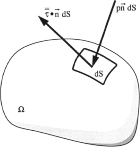
图2.2:作用在控制体表面元上的表面力。图例:\(\overline{\overline{\tau}}\cdot\vec{n}\,dS\)——黏性应力;\(p\vec{n}\,dS\)——压力;\(dS\)——面元;\(\Omega\)——控制体。
即固定在空间中的任意控制体\(\Omega\)内的动量守恒。en
for the momentum conservation inside an arbitrary control volume \(\Omega\) which is fixed in space.
2.2.3 The Energy Equation 能量方程[cfd-2-2-3]
我们在推导能量方程时所依据的基本原理是热力学第一定律。把它应用于图2.1所示的控制体,可以表述为:体积内总能量随时间的任何变化,都是由作用在该体积上的力的做功速率以及流入该体积的净热流引起的。流体单位质量的总能量\(E\),由其单位质量内能\(e\)加上单位质量动能\(|\vec{v}|^{2}/2\)而得到。因此,总能量可以写为en
The underlying principle that we will apply in the derivation of the energy equation, is the first law of thermodynamics. Applied to the control volume displayed in Fig. 2.1, it states that any changes in time of the total energy inside the volume are caused by the rate of work of forces acting on the volume and by the net heat flux into it. The total energy per unit mass \(E\) of a fluid is obtained by adding its internal energy per unit mass, \(e\), to its kinetic energy per unit mass \(|\vec{v}|^{2}/2\). Thus, we can write for the total energy
此情形下的守恒量是单位体积的总能量,即\(\rho E\)。它在体积\(\Omega\)内随时间的变化可表示为en
The conserved quantity is in this case the total energy per unit volume, i.e., \(\rho E\). Its variation in time within the volume \(\Omega\) can be expressed as
与连续方程和动量方程不同,这里出现了扩散通量。如前所述,它与单位质量守恒量的梯度成正比(Fick定律)。由于扩散通量\(\vec{F}_D\)是针对静止流体定义的,只有内能起作用,于是得到en
In contrast to the continuity and the momentum equation, there is now a diffusive flux. As we already stated, it is proportional to the gradient of the conserved quantity per unit mass (Fick's law). Since the diffusive flux \(\vec{F}_D\) is defined for a fluid at rest, only the internal energy becomes effective and we obtain
上式中,\(\gamma = c_p/c_v\)为比热系数之比,\(\kappa\)为热扩散率系数(thermal diffusivity coefficient)。扩散通量代表进入控制体热流的一部分,即由分子热传导引起的热扩散——由温度梯度导致的传热。因此,方程(2.7)通常写成Fourier热传导定律的形式,即en
In the above, \(\gamma = c_p/c_v\) is the ratio of specific heat coefficients, and \(\kappa\) denotes the thermal diffusivity coefficient. The diffusion flux represents one part of the heat flux into the control volume, namely the diffusion of heat due to molecular thermal conduction - heat transfer due to temperature gradients. Therefore, Equation (2.7) is in general written in the form of Fourier's law of heat conduction, i.e.,
其中\(k\)为热导率系数(thermal conductivity coefficient),\(T\)为绝对静温。en
with \(k\) standing for the thermal conductivity coefficient and \(T\) for the absolute static temperature.
进入有限控制体的净热流的另一部分,是由辐射的吸收或发射、或化学反应引起的体积加热。我们把热源——单位质量传热的时间变化率——记作\(\dot{q}_h\)。它与为动量方程引入的体力\(\vec{f}_e\)的做功速率一起,构成完整的体积源en
The other part of the net heat flux into the finite control volume consists of volumetric heating due to the absorption or emission of radiation, or due to chemical reactions. We will denote the heat sources - the time rate of heat transfer per unit mass - as \(\dot{q}_h\). Together with the rate of work done by the body forces \(\vec{f}_e\), which we have introduced for the momentum equation, it completes the volume sources
能量守恒中尚待确定的最后一项贡献是面源\(Q_S\)。它对应于压力以及切向和法向应力对流体微元做功的时间变化率(见图2.2),即en
The last contribution to the conservation of energy, which we have yet to determine, are the surface sources \(Q_S\). They correspond to the time rate of work done by the pressure as well as the shear and normal stresses on the fluid element (see Fig. 2.2), i.e.,
把上述所有贡献和各项整理起来,便得到能量守恒方程的表达式en
Sorting now all the above contributions and terms, we obtain for the energy conservation equation the expression
2.3 Viscous Stresses 黏性应力[cfd-2-3]
黏性应力源于流体与微元表面之间的摩擦,由应力张量\(\overline{\overline{\tau}}\)描述。在笛卡尔坐标系中,其一般形式为en
The viscous stresses, which originate from the friction between the fluid and the surface of an element, are described by the stress tensor \(\overline{\overline{\tau}}\). In Cartesian coordinates its general form is given by
按照惯例,记号\(\tau_{ij}\)表示该应力分量作用在垂直于\(i\)轴的平面上、方向沿\(j\)轴。分量\(\tau_{xx}\)、\(\tau_{yy}\)和\(\tau_{zz}\)代表法向应力,\(\overline{\overline{\tau}}\)的其余分量则分别代表切向应力。图2.3给出了四边形流体微元上的应力。可以看到,法向应力(图2.3a)试图使微元的各个面沿三个互相垂直的方向发生位移,而切向应力(图2.3b)则试图使微元发生剪切变形。en
The notation \(\tau_{ij}\) means by convention that the particular stress component affects a plane perpendicular to the \(i\)-axis, in the direction of the \(j\)-axis. The components \(\tau_{xx}\), \(\tau_{yy}\), and \(\tau_{zz}\) represent the normal stresses, the other components of \(\overline{\overline{\tau}}\) stand for the shear stresses, respectively. Figure 2.3 shows the stresses for a quadrilateral fluid element. One can notice that the normal stresses (Fig. 2.3a) try to displace the faces of the element in three mutually perpendicular directions, whereas the shear stresses (Fig. 2.3b) try to shear the element.
现在你可能会问,黏性应力是如何求得的。首先,它们取决于介质的动力学性质。对于空气或水这类流体,Isaac Newton指出切向应力与速度梯度成正比。因此,这类介质被称为牛顿流体(Newtonian fluid)。另一方面,诸如熔融塑料或血液等流体则表现出不同的行为——它们是非牛顿流体。但是,对于流体可以假设为牛顿流体的绝大多数实际问题,黏性应力张量的分量由如下关系定义[3], [4]en
You may ask now, how the viscous stresses are evaluated. First of all, they depend on the dynamical properties of the medium. For fluids like air or water, Isaac Newton stated that the shear stress is proportional to the velocity gradient. Therefore, medium of such a type is designated as Newtonian fluid. On the other hand, fluids like for example melted plastic or blood behave in a different manner - they are non-Newtonian fluids. But, for the vast majority of practical problems, where the fluid can be assumed to be Newtonian, the components of the viscous stress tensor are defined by the relations [3], [4]
其中\(\lambda\)为第二黏性系数(second viscosity),\(\mu\)为动力黏性系数(dynamic viscosity)。为方便起见,还可以定义所谓的运动黏性系数(kinematic viscosity),其公式为en
in which \(\lambda\) represents the second viscosity coefficient, and \(\mu\) denotes the dynamic viscosity coefficient. For convenience, we can also define the so-called kinematic viscosity coefficient, which is given by the formula
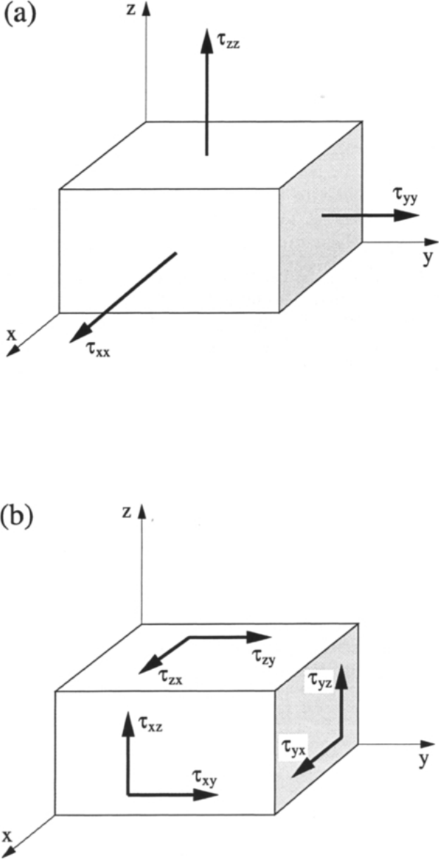
图2.3:作用在有限流体微元上的法向应力(a)与切向应力(b)。图例:(a)法向应力\(\tau_{xx}\)、\(\tau_{yy}\)、\(\tau_{zz}\);(b)切向应力\(\tau_{xy}\)、\(\tau_{xz}\)、\(\tau_{yx}\)、\(\tau_{yz}\)、\(\tau_{zx}\)、\(\tau_{zy}\)。
方程(2.15)中的表达式由英国人George Stokes在19世纪中叶导出。法向应力中的\(\mu(\partial u/\partial x)\)等项代表线膨胀率(linear dilatation)——形状的变化。另一方面,方程(2.15)中的项\((\lambda\,\mathrm{div}\,\vec{v})\)代表体积膨胀(volumetric dilatation)——体积的变化率,其本质是密度的变化。en
The expressions in Eq. (2.15) were derived by the Englishman George Stokes in the middle of the 19th century. The terms \(\mu(\partial u/\partial x)\), etc. in the normal stresses represent the rate of linear dilatation - a change in shape. On the other hand, the term \((\lambda\,\mathrm{div}\,\vec{v})\) in Eq. (2.15) represents volumetric dilatation - the rate of change in volume, which is in essence a change of the density.
除极高温度或极高压力的情形外,迄今尚无实验证据表明方程(2.17)中的Stokes假设不成立(参见文献[6]中的讨论)。因此,通常利用该假设从方程(2.15)中消去\(\lambda\)。于是,法向黏性应力为en
With the exception of extremely high temperatures or pressures, there is so far no experimental evidence that Stokes's hypothesis in Eq. (2.17) does not hold (see discussion in Ref. [6]). It is therefore generally used to eliminate \(\lambda\) from Eq. (2.15). Hence, we obtain for the normal viscous stresses
尚待确定的是作为流体状态函数的黏性系数\(\mu\)和热导率系数\(k\)。在连续介质力学的框架内,这只能依靠经验假设来完成。我们将在下一节回到这一问题。en
What remains to be determined are the viscosity coefficient \(\mu\) and the thermal conductivity coefficient \(k\) as functions of the state of the fluid. This can be done within the framework of continuum mechanics only on the basis of empirical assumptions. We shall return to this problem in the next section.
2.4 Complete System of the Navier-Stokes Equations 完整的Navier-Stokes方程组[cfd-2-4]
在前面几节中,我们分别导出了质量、动量和能量的守恒定律。现在,可以把它们汇集为一个方程组,以便更清楚地总览其中所含的各项。为此,我们回到向量量的一般守恒定律,即方程(2.2)。出于后面将会说明的原因,我们引入两个通量向量,即\(\vec{F}_c\)和\(\vec{F}_v\)。第一个向量\(\vec{F}_c\)与流体中物理量的对流输运有关,通常称为对流通量向量(vector of convective fluxes),尽管对动量方程和能量方程而言,它还分别包含压力项\(p\vec{n}\)(方程(2.5))和\(p\left(\vec{v}\cdot\vec{n}\right)\)(方程(2.11))。第二个通量向量称为黏性通量向量(vector of viscous fluxes)\(\vec{F}_v\),它包含黏性应力以及热扩散。此外,再定义一个源项\(\vec{Q}\),它涵盖由体力和体积加热引起的所有体积源。记住这些定义,并与单位法向量\(\vec{n}\)作标量积,我们就可以把方程(2.2)与方程(2.3)、(2.5)和(2.13)合并为en
In the previous sections, we have separately derived the conservation laws of mass, momentum and energy. Now, we can collect them into one system of equations in order to obtain a better overview of the various terms involved. For this purpose, we go back to the general conservation law for a vector quantity, which is expressed in Equation (2.2). For reasons to be explained later, we will introduce two flux vectors, namely \(\vec{F}_c\) and \(\vec{F}_v\). The first one, \(\vec{F}_c\), is related to the convective transport of quantities in the fluid. It is usually termed vector of convective fluxes, although for the momentum and the energy equation it also includes the pressure terms \(p\vec{n}\) (Eq. (2.5)) and \(p\left(\vec{v}\cdot\vec{n}\right)\) (Eq. (2.11)), respectively. The second flux vector - denoted the vector of viscous fluxes \(\vec{F}_v\), contains the viscous stresses as well as the heat diffusion. Additionally, let us define a source term \(\vec{Q}\), which comprises all volume sources due to body forces and volumetric heating. With all this in mind and conducting the scalar product with the unit normal vector \(\vec{n}\), we can cast Eq. (2.2) together with Equations (2.3), (2.5) and (2.13) into
所谓守恒变量(conservative variables)的向量\(\vec{W}\),在三维情形下由以下五个分量组成en
The vector of the so-called conservative variables \(\vec{W}\) consists in three dimensions of the following five components
对流通量向量为en
For the vector of convective fluxes we obtain
其中逆变速度(contravariant velocity)\(V\)——垂直于面元\(dS\)的速度——定义为速度向量与单位法向量的标量积,即en
with the contravariant velocity \(V\) - the velocity normal to the surface element \(dS\) - being defined as the scalar product of the velocity vector and the unit normal vector, i.e.,
其中en
where
它们是分别描述黏性应力做功和流体中热传导的各项。最后,源项为en
are terms describing the work of the viscous stresses and of the heat conduction in the fluid, respectively. Finally, the source term reads
对于牛顿流体,即当黏性应力满足方程(2.15)的关系时,上述方程组(方程(2.19)–(2.25))就称为Navier-Stokes方程(Navier-Stokes equations)。它们描述质量、动量和能量穿过固定在空间中的控制体\(\Omega\)之边界\(\partial\Omega\)的交换(通量)(见图2.1)。我们是按照守恒定律、以积分形式导出Navier-Stokes方程的。应用Gauss定理,方程(2.19)可以改写为微分形式[7]。由于微分形式在文献中经常出现,为完整起见将其收入附录(A.1)中。en
In the case of a Newtonian fluid, i.e., if the relations Eq. (2.15) for the viscous stresses are valid, the above system of equations (Eqs. (2.19)-(2.25)) is called the Navier-Stokes equations. They describe the exchange (flux) of mass, momentum and energy through the boundary \(\partial\Omega\) of a control volume \(\Omega\), which is fixed in space (see Fig. 2.1). We have derived the Navier-Stokes equations in integral formulation, in accordance with the conservation laws. Applying Gauss's theorem, Equation (2.19) can be re-written in differential form [7]. Since the differential form is often found in literature, it is for completeness included in the Appendix (A.1).
在某些情形下,例如在叶轮机械应用或地球物理中,控制体会绕某一轴(通常是稳定地)旋转。此时,需要把Navier-Stokes方程变换到旋转参考系(rotating frame of reference)中。其结果是,源项\(\vec{Q}\)必须补充由科里奥利力和离心力引起的影响[8]。所得形式的Navier-Stokes方程可参见附录(A.4)。另一些情形下,控制体可能发生平移或变形,例如在研究流固耦合(fluid-structure interaction)时就会出现这种情况。此时,Navier-Stokes方程(2.19)必须补充一个描述面元\(dS\)相对于固定坐标系之相对运动的项[9]。此外,还必须满足所谓的几何守恒定律(Geometric Conservation Law,GCL)[10]-[12]。相应的表述在附录(A.5)中给出。en
In some instances, for example in turbomachinery applications or geophysics, the control volume is rotating (usually steadily) about some axis. In such a case, the Navier-Stokes equations are transformed into a rotating frame of reference. As a consequence, the source term \(\vec{Q}\) has to be extended by the effects due to the Coriolis and the centrifugal force [8]. The resulting form of the Navier-Stokes equations may be found in the Appendix (A.4). In other cases, the control volume can be subject to translation or deformation. This happens, for instance, when fluid-structure interaction is investigated. Then, the Navier-Stokes equations (2.19) have to be extended by a term, which describes the relative motion of the surface element \(dS\) with respect to the fixed coordinate system [9]. Additionally, the so-called Geometric Conservation Law (GCL) has to be fulfilled [10]-[12]. We present the appropriate formulation in Section (A.5) of the Appendix.
在三维情形下,Navier-Stokes方程是关于五个守恒变量\(\rho\)、\(\rho u\)、\(\rho v\)、\(\rho w\)和\(\rho E\)的五个方程组成的方程组。但它们包含七个未知的流场变量,即:\(\rho\)、\(u\)、\(v\)、\(w\)、\(E\)、\(p\)和\(T\)。因此,我们必须补充两个附加方程,它们应当是状态变量之间的热力学关系。例如,把压力表示为密度和温度的函数,把内能或焓表示为压力和温度的函数。除此之外,还必须给出作为流体状态函数的黏性系数\(\mu\)和热导率系数\(k\),以使整个方程组封闭。显然,这些关系取决于所考虑的流体种类。下面我们将针对两种常见情形给出使方程封闭的方法。en
The Navier-Stokes equations represent in three dimensions a system of five equations for the five conservative variables \(\rho\), \(\rho u\), \(\rho v\), \(\rho w\), and \(\rho E\). But they contain seven unknown flow field variables, namely: \(\rho\), \(u\), \(v\), \(w\), \(E\), \(p\), and \(T\). Therefore, we have to supply two additional equations, which have to be thermodynamic relations between the state variables. For example, the pressure expressed as a function of the density and temperature, and the internal energy or the enthalpy given as a function of the pressure and temperature. Beyond this, we have to provide the viscosity coefficient \(\mu\) and the thermal conductivity coefficient \(k\) as functions of the state of the fluid, in order to close the entire system of equations. Clearly, the relationships depend on the kind of fluid being considered. In the following, we shall therefore show methods of closing the equations for two commonly encountered situations.
2.4.1 Formulation for a Perfect Gas 完全气体的形式[cfd-2-4-1]
其中\(R\)为比气体常数。焓由下式给出en
where \(R\) denotes the specific gas constant. The enthalpy results from
用守恒变量表示压力会带来方便。为此,需要把联系总焓与总能量的方程(2.12)与状态方程(2.26)结合起来。把表达式(2.27)代入焓,并利用定义en
It is convenient to express the pressure in terms of the conservative variables. For that purpose, we have to combine Equation (2.12), relating the total enthalpy to the total energy, together with the equation of state (2.26). Substituting expression (2.27) for the enthalpy and using the definitions
最终得到压力en
we finally obtain for the pressure
温度随后借助关系式(2.26)计算。对完全气体而言,动力黏性系数\(\mu\)强烈依赖于温度,而受压力的影响很弱。常用的公式是所谓的Sutherland公式。对空气的结果为(SI单位)en
The temperature is then calculated with the aid of the relationship Eq. (2.26). The coefficient of the dynamic viscosity \(\mu\) is, for a perfect gas, strongly dependent on temperature but only weakly dependent on pressure. The so-called Sutherland formula is frequently used. The result for air is (in SI units)
其中温度\(T\)以开尔文(K)为单位。于是,在\(T = 288\,\mathrm{K}\)时可得\(\mu = 1.78\cdot 10^{-5}\,\mathrm{kg/ms}\)。气体中热导率系数\(k\)对温度的依赖关系与\(\mu\)类似;相反,液体中\(k\)几乎为常数。因此,对空气通常采用关系式en
where the temperature \(T\) is in degree Kelvin (K). Thus, at \(T = 288\,\mathrm{K}\) one obtains \(\mu = 1.78\cdot 10^{-5}\,\mathrm{kg/ms}\). The temperature dependence of the thermal conductivity coefficient \(k\) resembles that of \(\mu\) in the case of gases. By contrast, \(k\) is virtually constant in the case of liquids. For this reason, the relationship
此外,通常还假定Prandtl数\(Pr\)在整个流场中为常数。对空气,Prandtl数取值\(Pr = 0.72\)。en
is generally used for air. In addition, it is commonly assumed that the Prandtl number \(Pr\) is constant in the entire flow field. For air, the Prandtl number takes the value \(Pr = 0.72\).
2.4.2 Formulation for a Real Gas 真实气体的形式[cfd-2-4-2]
当必须处理真实气体(real gas)时,问题变得更加复杂。原因在于,除流体动力学外,现在还必须对热力学过程和化学反应进行建模。真实气体流动的例子有:燃烧的模拟、再入飞行器的高超声速绕流,以及汽轮机内的流动。原则上,可以采取两种不同的方法来求解这一问题。第一种方法适用于气体处于化学平衡和热力学平衡的情形。这意味着存在唯一的状态方程,此时控制方程(2.19)保持不变,只是压力、温度、黏度等的数值要通过曲线拟合从查询表中插值得到[15]-[17]。但在实际中,气体更多是处于化学和/或热力学非平衡状态,必须相应地加以处理。en
The matter becomes more complicated when one has to deal with a real gas. The reason is that now we have to model a thermodynamic process and chemical reactions in addition to the fluid dynamics. Examples for a real gas flow are the simulation of combustion, the hypersonic flow past a re-entry vehicle, or the flow in a steam turbine. In principle, two different methods can be pursued to solve the problem. The first methodology is applicable in cases, where the gas is in chemical and in thermodynamical equilibrium. This implies that there is a unique equation of state. Then, the governing equations (2.19) remain unchanged. Only the values of pressure, temperature, viscosity, etc. are interpolated from lookup tables using curve fits [15]-[17]. But in practice, the gas is more often in chemical and/or thermodynamical non-equilibrium and has to be treated correspondingly.
为便于说明,考虑由\(N\)种不同组分组成的气体混合物。对于有限的Damköhler数——其定义为流动滞留时间与化学反应时间之比——必须在模型中纳入有限速率化学。该模型需要描述化学反应引起的组分的生成与消亡。下面我们进一步假定,流体动力学和化学反应的时间尺度与空间尺度都远大于热力学的相应尺度。于是,我们假定气体处于热力学平衡但化学非平衡状态。为了模拟这种气体混合物的行为,必须为\(N\)种组分补充\((N-1)\)个附加输运方程,从而扩展Navier-Stokes方程[18]-[23]。这样,我们得到形式上与方程(2.19)相同的方程组,但守恒变量向量\(\vec{W}\)、通量向量\(\vec{F}_c\)和\(\vec{F}_v\)以及源项\(\vec{Q}\)都被\((N-1)\)个组分方程所扩展。回顾表达式(2.20)至(2.25),守恒变量向量现在为en
Let us for illustration consider a gas mixture consisting of \(N\) different species. For a finite Damköhler number, which is defined as the ratio of flow-residence time to chemical-reaction time, we have to include finite-rate chemistry into our model. It has to describe the generation/destruction of species due to chemical reactions. In what follows, we will furthermore assume that the temporal and the spatial scales of fluid dynamics and of chemical reactions are much larger compared to those of thermodynamics. Thus, we suppose the gas is thermodynamically in equilibrium but chemically in non-equilibrium. In order to simulate the behaviour of such a gas mixture, the Navier-Stokes equations have to be augmented by \((N-1)\) additional transport equations for the \(N\) species [18]-[23]. Hence, we obtain formally the same system like Eq. (2.19), but now with the vectors of the conservative variables \(\vec{W}\), the flux vectors \(\vec{F}_c\) and \(\vec{F}_v\), as well as with the source term \(\vec{Q}\) extended by \((N-1)\) species equations. Recalling the expressions (2.20) to (2.25), the vector of the conservative variables reads now
对流通量向量和黏性通量向量则变换为en
The convective and the viscous flux vectors transform into
其中en
where
最后,源项现在变为en
Finally, the source term now becomes
在上述表达式(方程(2.32)–(2.35))中,\(Y_m\)表示质量分数,\(h_m\)为焓,\(D_m\)为组分\(m\)的有效二元扩散系数。此外,\(\dot{s}_m\)是化学反应引起的组分\(m\)的变化率。注意,混合物的总密度\(\rho\)等于各组分密度\(\rho Y_m\)之和。因此,由于总密度被视为独立变量,只剩下\((N-1)\)个独立的密度\(\rho Y_m\)。其余的质量分数\(Y_N\)由下式求得en
In the above expressions Eqs. (2.32)-(2.35), \(Y_m\) denotes the mass fraction, \(h_m\) the enthalpy, and \(D_m\) the effective binary diffusivity of species \(m\), respectively. Furthermore, \(\dot{s}_m\) is the rate of change of species \(m\) due to chemical reactions. Note that the total density \(\rho\) of the mixture is equal to the sum of the densities of the species \(\rho Y_m\). Therefore, since the total density is regarded as an independent quantity, there are only \((N-1)\) independent densities \(\rho Y_m\) left. The remaining mass fraction \(Y_N\) is obtained from
为了得到压力\(p\)的表达式,首先假定各组分的行为如同理想气体,即en
In order to find an expression for the pressure \(p\), we first assume that the individual species behave like ideal gases, i.e.,
其中\(R_u\)为普适气体常数,\(W_m\)为分子量。结合Dalton定律en
with \(R_u\) denoting the universal gas constant and \(W_m\) being the molecular weight, respectively. Together with Dalton's law,
可以写出en
we can write
气体混合物的内能\(e\)由方程(2.6)得到。方程(2.40)中的\(h^{0}_{f,m}\)、\(c_{p,m}\)和\(T_{ref}\)分别表示第\(m\)种组分的生成热、定压比热和参考温度。上述物理量以及各组分的焓、热导率\(k\)和动力黏性\(\mu\)的数值,都由曲线拟合确定[19], [21], [23]。en
The internal energy of the gas mixture \(e\) is obtained from Eq. (2.6). The quantities \(h^{0}_{f,m}\), \(c_{p,m}\), and \(T_{ref}\) in Eq. (2.40) denote the heat of formation, the specific heat at constant pressure, and the reference temperature of the \(m\)-th species, respectively. Values of the above quantities as well as of the thermal conductivity \(k\) and of the dynamic viscosity \(\mu\) of the species are determined from curve fits [19], [21], [23].
最后一个尚待建模的部分是方程(2.35)中的化学源项\(\dot{s}_m\)。对于包含\(N\)种组分、由\(N_R\)个基元反应构成的反应集,其速率方程可以写成如下一般形式en
The last part, which remains to be modelled, is the chemical source term \(\dot{s}_m\) in Eq. (2.35). The rate equations for a set of \(N_R\) elementary reactions involving \(N\) species can be written in the general form
在方程(2.41)中,\(\nu'_{lm}\)和\(\nu''_{lm}\)分别是组分\(m\)在第\(l\)个正反应和逆反应中的化学计量系数。此外,\(C_m\)表示组分\(m\)的摩尔浓度(\(C_m = \rho Y_m/W_m\)),而\(K_{fl}\)和\(K_{bl}\)分别表示第\(l\)个反应步骤的正反应和逆反应速率常数。它们由经验Arrhenius公式给出en
In the above Eq. (2.41), \(\nu'_{lm}\) and \(\nu''_{lm}\) are the stoichiometric coefficients for species \(m\) in the \(l\)-th forward and backward reaction, respectively. Furthermore, \(C_m\) stands for the molar concentration of species \(m\) (\(C_m = \rho Y_m/W_m\)), and finally \(K_{fl}\) and \(K_{bl}\), respectively, denote the forward and the backward reaction rate constants for the \(l\)-th reaction step. They are given by the empirical Arrhenius formulae
其中\(A_f\)和\(A_b\)为Arrhenius系数,\(E_f\)和\(E_b\)为活化能,\(B_f\)和\(B_b\)为常数。第\(l\)个反应引起的组分\(m\)摩尔浓度的变化率为en
where \(A_f\) and \(A_b\) are the Arrhenius coefficients, \(E_f\) and \(E_b\) represent the activation energies, and \(B_f\) as well as \(B_b\) are constants, respectively. The rate of change of molar concentration of species \(m\) by the \(l\)-th reaction is given by
真实气体的另一个实用例子是蒸汽的模拟,或者更有挑战性的、叶轮机械应用中湿蒸汽的模拟[25]-[32]。在后一种情形中,蒸汽与水滴混合,即所谓的多相流(multiphase flow);此时既可以求解一组附加的输运方程,也可以沿若干条流线追踪水滴。这类模拟在现代汽轮机叶栅设计中有着十分重要的应用。例如,对涡轮叶片绕流的分析有助于理解凝结引起的超临界激波以及流动不稳定性的产生,后者会使叶片装置承受额外的动态载荷并导致效率损失。en
Another practical example of real gas is the simulation of steam or, which is more demanding, of wet steam in turbomachinery applications [25]-[32]. In the later case, where the steam is mixed with water droplets, so that we speak of multiphase flow, it is either possible to solve an additional set of transport equations, or to trace the water droplets along a number of streamlines. These simulations have very important applications in the design of modern steam turbine cascades. The analysis of flow past turbine blades can for instance help to understand the occurrence of supercritical shocks by condensation and of flow instabilities, responsible for an additional dynamic load on the bladings and resulting in a loss of the efficiency.
2.4.3 Simplifications to the Navier-Stokes Equations Navier-Stokes方程的简化[cfd-2-4-3]
下面考虑Navier-Stokes方程(2.19)的三种常见简化。这里我们把注意力集中在每种近似背后的物理依据上。前两种简化形式的方程在附录中给出。en
In the following, we shall consider three common simplifications to the Navier-Stokes equations (2.19). We shall restrict our attention here to the physical reasoning behind each of the approximations. The equations for the first two simplified forms of the Navier-Stokes equations are provided in the Appendix.
Thin Shear Layer Approximation 薄剪切层近似
在模拟高雷诺数绕物体的流动时(即边界层相对于特征尺寸很薄时),可以对Navier-Stokes方程(2.19)进行简化。一个必要条件是不存在大面积的分离边界层。于是可以预期en
When simulating flows around bodies for high Reynolds numbers (i.e., when the boundary layer is thin with respect to a characteristic dimension), the Navier-Stokes equations (2.19) can be simplified. One necessary condition is that there is no large area of separated boundary layer. It can then be anticipated that
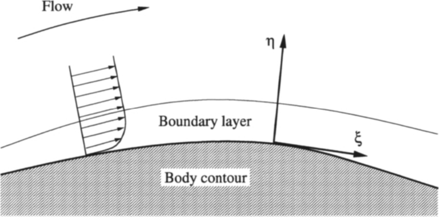
图2.4:薄边界层的表示。图例:Flow——流动;Boundary layer——边界层;Body contour——物面轮廓;\(\eta\)、\(\xi\)——贴体曲线坐标。
只有垂直于物体表面方向(图2.4中的\(\eta\)方向)的流动参量梯度才对黏性应力有贡献[33], [34]。另一方面,在其他坐标方向(图2.4中的\(\xi\)方向)上的梯度,在计算切向应力张量(方程(2.14, 2.15))时被忽略。这就是所谓的Navier-Stokes方程薄剪切层(Thin Shear Layer,TSL)近似。采用TSL修正的动机在于:黏性项的数值计算代价更低,同时在假设范围内解仍保持足够的精度。从实用的角度看,TSL近似也是合理的。在高雷诺数流动中,为了恰当地分辨边界层,网格在壁面法向必须非常细;而受计算机内存和速度的限制,其他方向的网格只能粗得多。这又使得梯度计算在这些方向上的数值精度明显低于法向。为完整起见,TSL方程在附录(A.6)中给出。由于二次流(例如叶排中的二次流)无法被恰当分辨,TSL简化通常只用于外流空气动力学。en
only the gradients of the flow quantities in the normal direction to the surface of the body (\(\eta\)-direction in Fig. 2.4) contribute to the viscous stresses [33], [34]. On the other hand, the gradients in the other coordinate directions (\(\xi\) in Fig. 2.4) are neglected in the evaluation of the shear stress tensor (Eqs. (2.14, 2.15)). We speak here of the so-called Thin Shear Layer (TSL) approximation of the Navier-Stokes equations. The motivation for the TSL modification is that the numerical evaluation of the viscous terms becomes computationally less expensive, but, within the assumptions, the solution remains sufficiently accurate. The TSL approximation can also be justified from a practical point of view. In the case of high Reynolds number flows, the grid has to be very fine in the wall normal direction in order to resolve the boundary layer properly. Because of the limited computer memory and speed, much coarser grid has to be generated in the other directions. This in turn results in significantly lower numerical accuracy of the gradient evaluation compared to the normal direction. The TSL equations are for completeness presented in the Appendix (A.6). Due to the fact that secondary flow (e.g., like in a blade row) cannot be resolved appropriately, the TSL simplification is usually applied only in external aerodynamics.
Parabolised Navier-Stokes Equations 抛物化Navier-Stokes方程
在满足以下三个条件的情况下:
- 流动是定常的(即\(\partial\vec{W}/\partial t = 0\));
- 流体主要沿一个主流方向运动(例如不得出现边界层分离);
- 横流分量可以忽略;
en
In cases, where the following three conditions are fulfilled:
- the flow is steady (i.e. \(\partial\vec{W}/\partial t = 0\)),
- the fluid moves predominantly in one main direction (e.g., there must be no boundary layer separation),
- the cross-flow components are negligible,
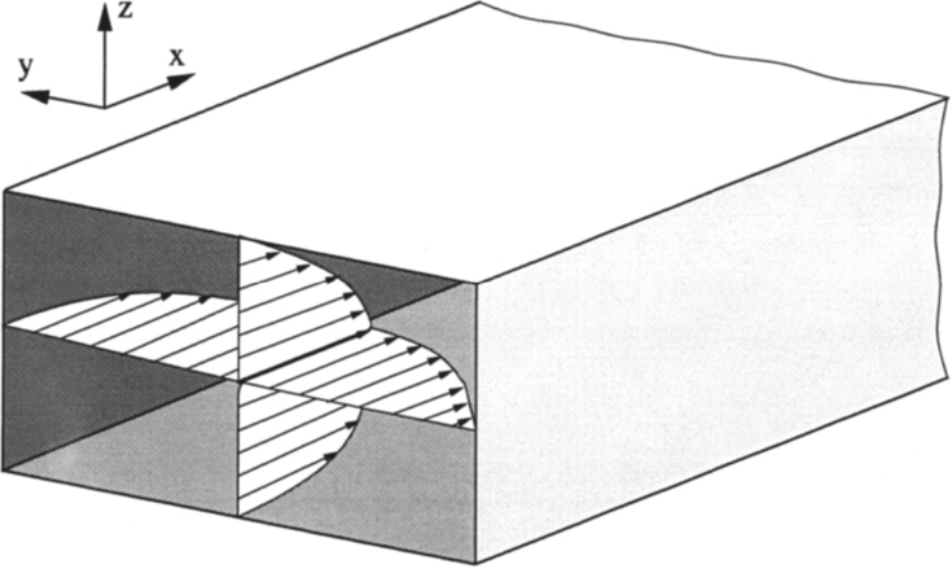
图2.5:管道内流——抛物化Navier-Stokes方程。
控制方程(2.19)可以简化为所谓的抛物化Navier-Stokes(Parabolised Navier-Stokes,PNS)方程[8], [35]-[37]。上述条件允许我们在黏性应力项(方程(2.15))中把\(u\)、\(v\)和\(w\)沿流向的导数取为零。此外,黏性应力张量\(\overline{\overline{\tau}}\)的分量、其做功项(\(\overline{\overline{\tau}}\cdot\vec{v}\))以及热传导\(k\nabla T\)在流向的分量,都从方程(2.23)的黏性通量向量中略去。连续方程以及对流通量(方程(2.21))保持不变。细节请参见附录(A.7)。考虑图2.5所示的情景,其中主流方向与\(x\)坐标一致,可以证明PNS近似导出一组抛物型/椭圆型混合的方程。具体而言,流向动量方程与能量方程一起成为抛物型方程,因此可以沿\(x\)方向推进求解;而\(y\)方向和\(z\)方向的动量方程是椭圆型的,必须在每个\(x\)平面内迭代求解。于是,PNS方法的主要好处在于流动求解复杂度的大幅降低——从完整的三维场变成一系列二维问题。抛物化Navier-Stokes方程的典型应用包括管道内的内流计算,以及利用空间推进方法模拟定常超声速流动[38]-[41]。en
the governing equations (2.19)) can be simplified to a form called the Parabolised Navier-Stokes (PNS) equations [8], [35]-[37]. The above conditions allow us to set the derivatives of \(u\), \(v\), and \(w\) with respect to the streamwise direction to zero in the viscous stress terms (Eq. (2.15)). Furthermore, the components of the viscous stress tensor \(\overline{\overline{\tau}}\), of the work performed by it (\(\overline{\overline{\tau}}\cdot\vec{v}\)), and of the heat conduction \(k\nabla T\) in the streamwise direction are dropped from the viscous flux vector in Eq. (2.23). The continuity equation, as well as the convective fluxes (Eq. (2.21)) remain unchanged. For details, the reader is referred to the Appendix (A.7). Considering the situation sketched in Fig. 2.5, where the main flow direction coincides with the \(x\) coordinate, it can be shown that the PNS approximation leads to a mixed set of parabolic / elliptic equations. Namely, the momentum equation in the flow direction becomes parabolic together with the energy equation, and hence they can be solved by marching in the \(x\)-direction. The momentum equations in the \(y\)- and in the \(z\)-direction are elliptic and they have to be solved iteratively in each \(x\)-plane. Thus, the main benefit of the PNS approach is in the largely reduced complexity of the flow solution - from a complete 3-D field to a sequence of 2-D problems. A typical application of the parabolised Navier-Stokes equations is the calculation of internal flows in ducts and in pipes, and also the simulation of steady supersonic flows using the space-marching method [38]-[41].
Euler Equations 欧拉方程
如前所述,Navier-Stokes方程描述黏性流体的行为。在许多情形下,完全忽略黏性效应是一种有效的近似,例如高雷诺数流动,其边界层相对于物体尺寸非常薄。此时,我们可以简单地从方程(2.19)中略去黏性通量向量\(\vec{F}_v\)。于是得到en
As we have seen, the Navier-Stokes equations describe the behaviour of a viscous fluid. In many instances, it is a valid approximation to neglect the viscous effects completely, like for example for high Reynolds-number flows, where the boundary layer is very thin compared to the dimensions of the body. In such cases, we can simply omit the vector of viscous fluxes, \(\vec{F}_v\), from the Equations (2.19). Thus, we are left with
其余各项仍由与前面相同的关系式(2.20)–(2.22)以及方程(2.25)给出。这种简化形式的控制方程称为欧拉方程(Euler equations)。它们描述无黏流体中流动物理量的纯对流。如果像上面那样以守恒形式表述欧拉方程,它们便能准确刻画激波、膨胀波以及三角翼(具有尖锐前缘)上的涡等重要现象。此外,欧拉方程在过去——并且至今仍然——是发展离散化方法和边界条件的基础。en
The remaining terms are given by the same relations (2.20)-(2.22) and Eq. (2.25) as before. This simplified form of the governing equations is called the Euler equations. They describe the pure convection of flow quantities in an inviscid fluid. If the Euler equations are formulated in conservative way (like above), they allow for accurate representation of such important phenomena like shocks, expansion waves and vortices over delta wings (with sharp leading edges). Furthermore, the Euler equations served in the past - and still do - as the basis for the development of discretisation methods and boundary conditions.
然而,应当指出,如今由于即使是个人计算机也具备的强大计算能力,以及对模拟质量要求的不断提高,欧拉方程已只是相对偶尔地用于流动计算。en
However, it should be noted that today, due to the computational power of even personal computers and due to the increased demands on the quality of the simulations, the Euler equations are only relatively seldom employed for flow computations.