2.4.3 Simplifications to the Navier-Stokes Equations Navier-Stokes方程的简化[cfd-2-4-3]
下面考虑Navier-Stokes方程(2.19)的三种常见简化。这里我们把注意力集中在每种近似背后的物理依据上。前两种简化形式的方程在附录中给出。en
In the following, we shall consider three common simplifications to the Navier-Stokes equations (2.19). We shall restrict our attention here to the physical reasoning behind each of the approximations. The equations for the first two simplified forms of the Navier-Stokes equations are provided in the Appendix.
Thin Shear Layer Approximation 薄剪切层近似
在模拟高雷诺数绕物体的流动时(即边界层相对于特征尺寸很薄时),可以对Navier-Stokes方程(2.19)进行简化。一个必要条件是不存在大面积的分离边界层。于是可以预期en
When simulating flows around bodies for high Reynolds numbers (i.e., when the boundary layer is thin with respect to a characteristic dimension), the Navier-Stokes equations (2.19) can be simplified. One necessary condition is that there is no large area of separated boundary layer. It can then be anticipated that
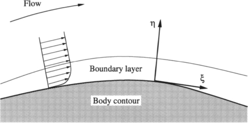
图2.4:薄边界层的表示。图例:Flow——流动;Boundary layer——边界层;Body contour——物面轮廓;\(\eta\)、\(\xi\)——贴体曲线坐标。
只有垂直于物体表面方向(图2.4中的\(\eta\)方向)的流动参量梯度才对黏性应力有贡献[33], [34]。另一方面,在其他坐标方向(图2.4中的\(\xi\)方向)上的梯度,在计算切向应力张量(方程(2.14, 2.15))时被忽略。这就是所谓的Navier-Stokes方程薄剪切层(Thin Shear Layer,TSL)近似。采用TSL修正的动机在于:黏性项的数值计算代价更低,同时在假设范围内解仍保持足够的精度。从实用的角度看,TSL近似也是合理的。在高雷诺数流动中,为了恰当地分辨边界层,网格在壁面法向必须非常细;而受计算机内存和速度的限制,其他方向的网格只能粗得多。这又使得梯度计算在这些方向上的数值精度明显低于法向。为完整起见,TSL方程在附录(A.6)中给出。由于二次流(例如叶排中的二次流)无法被恰当分辨,TSL简化通常只用于外流空气动力学。en
only the gradients of the flow quantities in the normal direction to the surface of the body (\(\eta\)-direction in Fig. 2.4) contribute to the viscous stresses [33], [34]. On the other hand, the gradients in the other coordinate directions (\(\xi\) in Fig. 2.4) are neglected in the evaluation of the shear stress tensor (Eqs. (2.14, 2.15)). We speak here of the so-called Thin Shear Layer (TSL) approximation of the Navier-Stokes equations. The motivation for the TSL modification is that the numerical evaluation of the viscous terms becomes computationally less expensive, but, within the assumptions, the solution remains sufficiently accurate. The TSL approximation can also be justified from a practical point of view. In the case of high Reynolds number flows, the grid has to be very fine in the wall normal direction in order to resolve the boundary layer properly. Because of the limited computer memory and speed, much coarser grid has to be generated in the other directions. This in turn results in significantly lower numerical accuracy of the gradient evaluation compared to the normal direction. The TSL equations are for completeness presented in the Appendix (A.6). Due to the fact that secondary flow (e.g., like in a blade row) cannot be resolved appropriately, the TSL simplification is usually applied only in external aerodynamics.
Parabolised Navier-Stokes Equations 抛物化Navier-Stokes方程
在满足以下三个条件的情况下:
- 流动是定常的(即\(\partial\vec{W}/\partial t = 0\));
- 流体主要沿一个主流方向运动(例如不得出现边界层分离);
- 横流分量可以忽略;
en
In cases, where the following three conditions are fulfilled:
- the flow is steady (i.e. \(\partial\vec{W}/\partial t = 0\)),
- the fluid moves predominantly in one main direction (e.g., there must be no boundary layer separation),
- the cross-flow components are negligible,
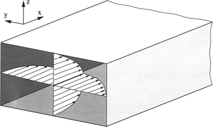
图2.5:管道内流——抛物化Navier-Stokes方程。
控制方程(2.19)可以简化为所谓的抛物化Navier-Stokes(Parabolised Navier-Stokes,PNS)方程[8], [35]-[37]。上述条件允许我们在黏性应力项(方程(2.15))中把\(u\)、\(v\)和\(w\)沿流向的导数取为零。此外,黏性应力张量\(\overline{\overline{\tau}}\)的分量、其做功项(\(\overline{\overline{\tau}}\cdot\vec{v}\))以及热传导\(k\nabla T\)在流向的分量,都从方程(2.23)的黏性通量向量中略去。连续方程以及对流通量(方程(2.21))保持不变。细节请参见附录(A.7)。考虑图2.5所示的情景,其中主流方向与\(x\)坐标一致,可以证明PNS近似导出一组抛物型/椭圆型混合的方程。具体而言,流向动量方程与能量方程一起成为抛物型方程,因此可以沿\(x\)方向推进求解;而\(y\)方向和\(z\)方向的动量方程是椭圆型的,必须在每个\(x\)平面内迭代求解。于是,PNS方法的主要好处在于流动求解复杂度的大幅降低——从完整的三维场变成一系列二维问题。抛物化Navier-Stokes方程的典型应用包括管道内的内流计算,以及利用空间推进方法模拟定常超声速流动[38]-[41]。en
the governing equations (2.19)) can be simplified to a form called the Parabolised Navier-Stokes (PNS) equations [8], [35]-[37]. The above conditions allow us to set the derivatives of \(u\), \(v\), and \(w\) with respect to the streamwise direction to zero in the viscous stress terms (Eq. (2.15)). Furthermore, the components of the viscous stress tensor \(\overline{\overline{\tau}}\), of the work performed by it (\(\overline{\overline{\tau}}\cdot\vec{v}\)), and of the heat conduction \(k\nabla T\) in the streamwise direction are dropped from the viscous flux vector in Eq. (2.23). The continuity equation, as well as the convective fluxes (Eq. (2.21)) remain unchanged. For details, the reader is referred to the Appendix (A.7). Considering the situation sketched in Fig. 2.5, where the main flow direction coincides with the \(x\) coordinate, it can be shown that the PNS approximation leads to a mixed set of parabolic / elliptic equations. Namely, the momentum equation in the flow direction becomes parabolic together with the energy equation, and hence they can be solved by marching in the \(x\)-direction. The momentum equations in the \(y\)- and in the \(z\)-direction are elliptic and they have to be solved iteratively in each \(x\)-plane. Thus, the main benefit of the PNS approach is in the largely reduced complexity of the flow solution - from a complete 3-D field to a sequence of 2-D problems. A typical application of the parabolised Navier-Stokes equations is the calculation of internal flows in ducts and in pipes, and also the simulation of steady supersonic flows using the space-marching method [38]-[41].
Euler Equations 欧拉方程
如前所述,Navier-Stokes方程描述黏性流体的行为。在许多情形下,完全忽略黏性效应是一种有效的近似,例如高雷诺数流动,其边界层相对于物体尺寸非常薄。此时,我们可以简单地从方程(2.19)中略去黏性通量向量\(\vec{F}_v\)。于是得到en
As we have seen, the Navier-Stokes equations describe the behaviour of a viscous fluid. In many instances, it is a valid approximation to neglect the viscous effects completely, like for example for high Reynolds-number flows, where the boundary layer is very thin compared to the dimensions of the body. In such cases, we can simply omit the vector of viscous fluxes, \(\vec{F}_v\), from the Equations (2.19). Thus, we are left with
其余各项仍由与前面相同的关系式(2.20)–(2.22)以及方程(2.25)给出。这种简化形式的控制方程称为欧拉方程(Euler equations)。它们描述无黏流体中流动物理量的纯对流。如果像上面那样以守恒形式表述欧拉方程,它们便能准确刻画激波、膨胀波以及三角翼(具有尖锐前缘)上的涡等重要现象。此外,欧拉方程在过去——并且至今仍然——是发展离散化方法和边界条件的基础。en
The remaining terms are given by the same relations (2.20)-(2.22) and Eq. (2.25) as before. This simplified form of the governing equations is called the Euler equations. They describe the pure convection of flow quantities in an inviscid fluid. If the Euler equations are formulated in conservative way (like above), they allow for accurate representation of such important phenomena like shocks, expansion waves and vortices over delta wings (with sharp leading edges). Furthermore, the Euler equations served in the past - and still do - as the basis for the development of discretisation methods and boundary conditions.
然而,应当指出,如今由于即使是个人计算机也具备的强大计算能力,以及对模拟质量要求的不断提高,欧拉方程已只是相对偶尔地用于流动计算。en
However, it should be noted that today, due to the computational power of even personal computers and due to the increased demands on the quality of the simulations, the Euler equations are only relatively seldom employed for flow computations.