9.3.1 Central IRS on Structured Grids 结构网格上的中心IRS[cfd-9-3-1]

隐式残差光顺的标准形式在三维情形下为en

The standard formulation of the implicit residual smoothing reads in 3D

\begin{aligned} -\epsilon^I\vec{R}^{*}_{I-1,J,K} + \left(1 + 2\epsilon^I\right)\vec{R}^{*}_{I,J,K} - \epsilon^I\vec{R}^{*}_{I+1,J,K} &= \vec{R}_{I,J,K}\\ -\epsilon^J\vec{R}^{**}_{I,J-1,K} + \left(1 + 2\epsilon^J\right)\vec{R}^{**}_{I,J,K} - \epsilon^J\vec{R}^{**}_{I,J+1,K} &= \vec{R}^{*}_{I,J,K}\\ -\epsilon^K\vec{R}^{***}_{I,J,K-1} + \left(1 + 2\epsilon^K\right)\vec{R}^{***}_{I,J,K} - \epsilon^K\vec{R}^{***}_{I,J,K+1} &= \vec{R}^{**}_{I,J,K}\ , \end{aligned} \tag{9.5}

其中 $\vec{R}^{*}_{I,J,K}$ 、 $\vec{R}^{**}_{I,J,K}$ 和 $\vec{R}^{***}_{I,J,K}$ 分别表示 $$I$$ 、 $$J$$ 、 $$K$$ 方向上光顺后的残差。参数 $\epsilon^I$ 、 $\epsilon^J$ 和 $\epsilon^K$ 表示三个计算坐标方向上的光顺系数。式(9.5)中的隐式算子类似于二阶中心差分，因此称为中心隐式残差光顺（Central Implicit Residual Smoothing，CIRS）。式(9.5)中的隐式方程组用求三对角矩阵之逆的Thomas算法求解。en

where $\vec{R}^{*}_{I,J,K}$ , $\vec{R}^{**}_{I,J,K}$ , and $\vec{R}^{***}_{I,J,K}$ denote the smoothed residuals in $$I$$ -, $$J$$ -, and $$K$$ -direction, respectively. The parameters $\epsilon^I$ , $\epsilon^J$ , and $\epsilon^K$ stand for the smoothing coefficients in the three computational coordinates. The implicit operator in Eq. (9.5) resembles second-order central difference. The term Central Implicit Residual Smoothing (CIRS) is therefore used. The implicit system in Eq. (9.5) is solved by the Thomas algorithm for the inversion of tridiagonal matrices.

光顺系数通常定义为对流通量雅可比矩阵谱半径的函数[11]。其目的是在每个坐标方向上只施加为保持稳定性与良好误差阻尼所必需的光顺量。文献[12]针对二维情形给出了一个合适的公式en

The smoothing coefficients are usually defined as functions of spectral radii of the convective flux Jacobians [11]. The purpose is to apply only as much smoothing in each coordinate direction as it is necessary for stability and good error damping. A suitable formula for 2D was suggested in [12]

\begin{aligned} \epsilon^I &= \max\left\{\frac{1}{4}\left[\left(\frac{\sigma^{*}}{\sigma}\,\frac{1}{1 + \Psi r}\right)^{2} - 1\right],\,0\right\}\\ \epsilon^J &= \max\left\{\frac{1}{4}\left[\left(\frac{\sigma^{*}}{\sigma}\,\frac{1}{1 + \Psi/r}\right)^{2} - 1\right],\,0\right\}\ . \end{aligned} \tag{9.6}

这里， $\sigma^{*}/\sigma$ 表示光顺格式与未光顺格式的CFL数之比。变量 $$r$$ 表示对流通量谱半径之比（式(4.53)），即 $r = \hat{\Lambda}_c^{J}/\hat{\Lambda}_c^{I}$ 。参数 $\Psi \approx 0.125$ 保证光顺操作的线性稳定性。en

Here, $\sigma^{*}/\sigma$ denotes the ratio of the CFL numbers of the smoothed and unsmoothed scheme. The variable $$r$$ stands for the ratio of the convective spectral radii (Eq. (4.53)), i.e., $r = \hat{\Lambda}_c^{J}/\hat{\Lambda}_c^{I}$ . The parameter $\Psi \approx 0.125$ ensures linear stability of the smoothing operation.

在三维情形下，可以用与式(9.6)类似的表达式来计算光顺系数[12]en

In 3D, the smoothing coefficients can be evaluated using an expression similar to Eq. (9.6) [12]

\begin{aligned} \epsilon^I &= \max\left\{\frac{1}{4}\left[\left(\frac{\sigma^{*}}{\sigma}\,\frac{1}{1 + \Psi\left(r^{JI} + r^{KI}\right)}\right)^{2} - 1\right],\,0\right\}\\ \epsilon^J &= \max\left\{\frac{1}{4}\left[\left(\frac{\sigma^{*}}{\sigma}\,\frac{1}{1 + \Psi\left(r^{KJ} + r^{IJ}\right)}\right)^{2} - 1\right],\,0\right\}\\ \epsilon^K &= \max\left\{\frac{1}{4}\left[\left(\frac{\sigma^{*}}{\sigma}\,\frac{1}{1 + \Psi\left(r^{IK} + r^{JK}\right)}\right)^{2} - 1\right],\,0\right\}\ , \end{aligned} \tag{9.7}

其中en

where

r^{JI} = \hat{\Lambda}_c^{J}/\hat{\Lambda}_c^{I}\,, \qquad r^{KI} = \hat{\Lambda}_c^{K}/\hat{\Lambda}_c^{I}\,, \tag{4}

等等。参数 $\Psi$ 的典型取值为0.0625。en

etc. The typical value of the parameter $\Psi$ is 0.0625.

CFL数之比 $\sigma^{*}/\sigma$ 的最大值取决于光顺系数的取值以及空间离散格式的类型。对于中心格式（4.3.1小节），该比值由下式给出en

The maximum of the ratio of the CFL numbers $\sigma^{*}/\sigma$ depends on the value of the smoothing coefficient and on the type of the spatial discretisation scheme. In the case of the central scheme (Subsection 4.3.1), the ratio is given by

\frac{\sigma^{*}}{\sigma} \le \sqrt{1 + 4\epsilon}\,. \tag{9.8}

实际中，可以达到 $\sigma^{*}/\sigma \approx 2$ （ $\epsilon = 0.8$ ）。更高的比值会削弱时间推进格式的阻尼能力。对于上风空间离散，不存在像式(9.8)这样简单的条件，因为 $\sigma^{*}/\sigma$ 的最大值还与各级系数有关。但通常，无黏流动的CFL数（见表6.1和表6.2）可以提高约两倍，黏性流动（采用表6.2中的混合格式）最多可提高约五倍。图9.2和图9.3展示了中心IRS对结构网格上无黏流动与黏性流动收敛的影响。比较按CPU时间进行，以计入IRS带来的额外计算量。可以看到，求解时间可以显著缩短，对黏性流动尤其明显。不过，当IRS与多重网格（9.4节）联合使用时，还能获得更大的节省。en

In practice, value of $\sigma^{*}/\sigma \approx 2$ can be reached ( $\epsilon = 0.8$ ). Higher ratios reduce the damping of the time-stepping scheme. There is no such simple condition like (9.8) for the upwind spatial discretisation since the maximum of $\sigma^{*}/\sigma$ depends also on the stage coefficients. But normally, the CFL number (see Tables 6.1 and 6.2) can be raised by about factor two for inviscid and up to factor five for viscous flows (using the hybrid scheme from Table 6.2). Figures 9.2 and 9.3 demonstrate the effect of the central IRS on the convergence for an inviscid and viscous flow on structured grids. The comparison is done in terms of the CPU time, in order to account for the additional numerical effort due to the IRS. As we can see, the solution time can be significantly reduced especially for a viscous flow. Even larger savings can be however realised when the IRS is employed together with multigrid (Section 9.4).

图9.2:结构网格上无黏跨声速流动有/无IRS时收敛历史的比较

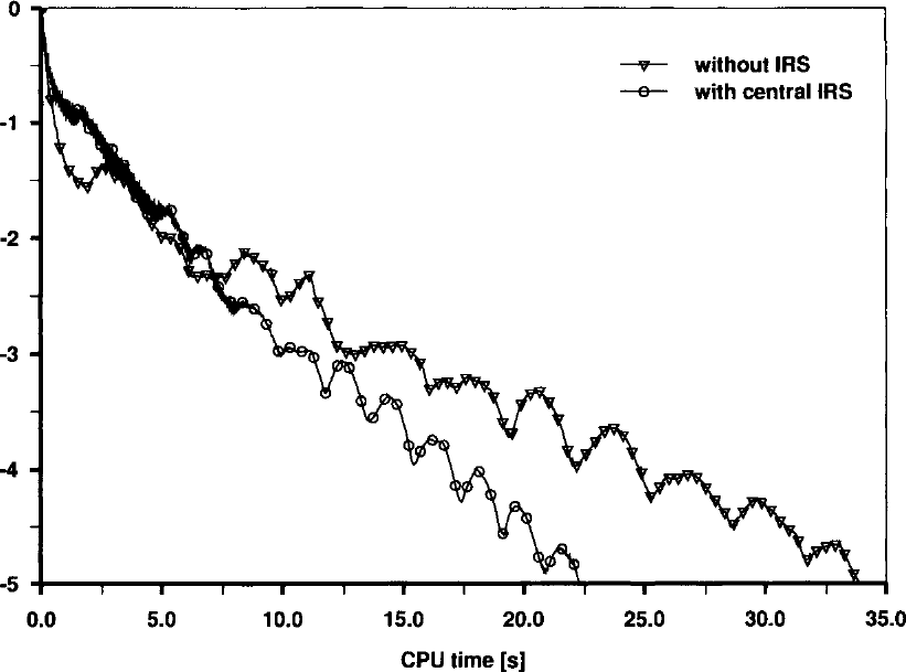
图9.2:结构网格上无黏跨声速流动有/无IRS时收敛历史的比较。纵轴:log(res)(残差的对数);横轴:CPU时间(CPU time [s]);图例:without IRS——无IRS;with central IRS——有中心IRS。

图9.3:结构网格上黏性亚声速流动有/无IRS时收敛历史的比较

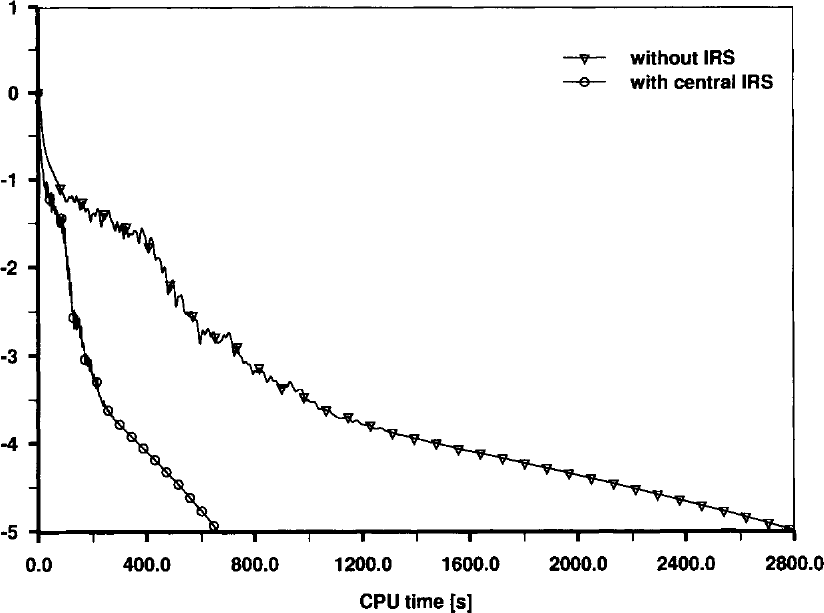
图9.3:结构网格上黏性亚声速流动有/无IRS时收敛历史的比较。纵轴:log(res)(残差的对数);横轴:CPU时间(CPU time [s]);图例:without IRS——无IRS;with central IRS——有中心IRS。

式(6.18)中由黏性谱半径 $\hat{\Lambda}_v$ 造成的时间步长限制，可以借助隐式残差光顺来补偿。最大时间步长按式(6.14)计算，但不包含 $\hat{\Lambda}_v$ 。在黏性谱半径占主导的流动区域，用较大的系数 $\epsilon^I$ 、 $\epsilon^J$ 、 $\epsilon^K$ 进行光顺。基于黏性谱半径的光顺系数可由文献[12]、[13]中的公式计算en

The limitation of the time step due to the viscous spectral radius $\hat{\Lambda}_v$ in Eq. (6.18) can be offset with the aid of the implicit residual smoothing. The maximum time step is calculated according to the formula (6.14) without $\hat{\Lambda}_v$ . In flow regions where the viscous spectral radius dominates, smoothing is carried out using higher coefficients $\epsilon^I$ , $\epsilon^J$ , $\epsilon^K$ . Smoothing coefficients based on the viscous spectral radii can be computed from [12], [13]

\begin{aligned} \epsilon_v^I &= C\left(\frac{\sigma^{*}}{\sigma}\right)\frac{\hat{\Lambda}_v^I}{\hat{\Lambda}_c^I + \hat{\Lambda}_c^J + \hat{\Lambda}_c^K}\\ \epsilon_v^J &= C\left(\frac{\sigma^{*}}{\sigma}\right)\frac{\hat{\Lambda}_v^J}{\hat{\Lambda}_c^I + \hat{\Lambda}_c^J + \hat{\Lambda}_c^K}\\ \epsilon_v^K &= C\left(\frac{\sigma^{*}}{\sigma}\right)\frac{\hat{\Lambda}_v^K}{\hat{\Lambda}_c^I + \hat{\Lambda}_c^J + \hat{\Lambda}_c^K}\ , \end{aligned} \tag{9.9}

其中常数 $C \approx 5/4$ 。然后取式(9.7)与式(9.9)中系数的最大值作为最终的光顺系数。en

where the constant $C \approx 5/4$ . The maximum of the coefficients from Eqs. (9.7) and (9.9) is then taken as the resulting smoothing coefficient.