4.3.5 Limiter Functions 限制器函数[cfd-4-3-5]
二阶及更高阶的上风空间离散需要使用所谓的限制器(limiter)或限制器函数(limiter function)ï¼以防止在大梯度区域(如激波处)产生振荡和虚假解。因此ï¼我们至少要寻找保持单调性(monotonicity preserving)的格式。这意味着流场中的极大值必须不增ï¼极小值必须不减ï¼且时间演化过程中不得产生新的局部极值;换言之ï¼若初始数据单调ï¼则解必须保持单调。保持单调性格式的相当苛刻的条件(或TVD格式更严格的条件)常常被放弃ï¼转而采用局部极值减小(Local Extremum Diminishing,LED)条件[60]。此时ï¼只要求包含在模板之内的局部极值减小。en
Second- and higher-order upwind spatial discretisations require the use of so-called limiters or limiter functions in order to prevent the generation of oscillations and spurious solutions in regions with large gradients (e.g., at shocks). Hence, what we are looking for is at least a monotonicity preserving scheme. This means that maxima in the flow field must be non-increasing, minima non-decreasing, and no new local extrema may be created during the time evolution. Or in other words, if the initial data is monotone then the solution has to remain monotone. The rather stringent conditions for monotonicity preserving schemes (or the more rigorous ones for TVD schemes) are often given up in favour of the Local Extremum Diminishing (LED) conditions [60]. Here, a local extremum contained only within the stencil has to decrease.
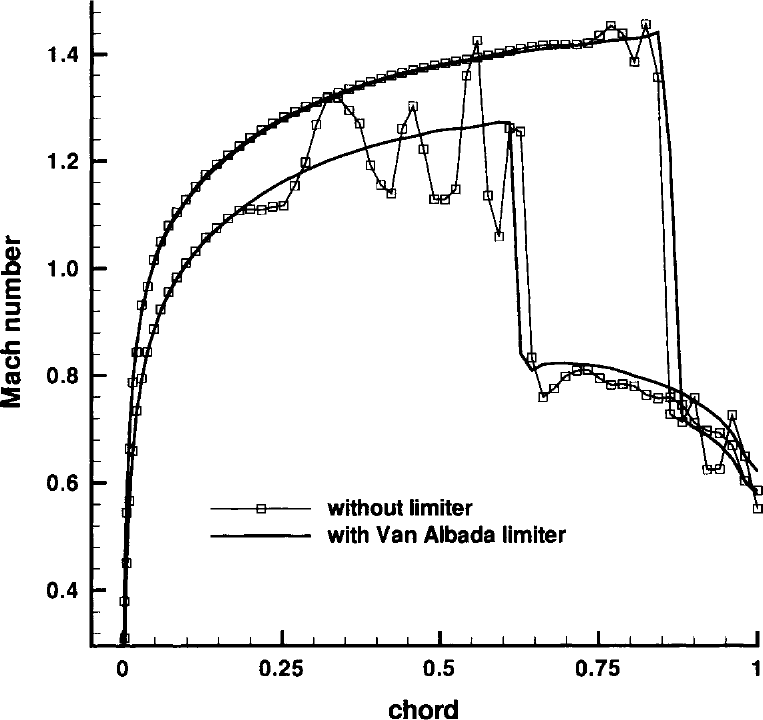
图4.10:有与无限制器的无黏跨声速流动计算比较。NACA 0012翼型,\(M_\infty\) = 0.85,\(\alpha\) = 1°。图例:纵轴为马赫数(Mach number)ï¼横轴为弦向位置(chord);带空心方块的折线为无限制器(without limiter)的结果ï¼实线为采用Van Albada限制器(with Van Albada limiter)的结果。
然而ï¼根据Godunov定理ï¼高阶线性格式(如MUSCL方法)不可能保持单调性[90]。因此ï¼必须采用非线性限制器函数来构造保持单调性或TVD的离散。图4.10演示了这一点:用方程(4.98)的上风TVD格式ï¼分别在有与无限制器的条件下计算NACA 0012翼型的二维跨声速流动。可以清楚看到ï¼无限制器时ï¼解在翼型上、下表面激波附近出现大幅振荡;而在远离激波处ï¼带限制器与不带限制器的解几乎相同。en
However, due to Godunov's theorem there is no possibility for a higher-order linear scheme (such as the MUSCL approach) to be monotonicity preserving [90]. It is therefore necessary to employ non-linear limiter functions in order to construct a monotonicity preserving or a TVD discretisation. This is demonstrated in Fig. 4.10, where the upwind TVD scheme of Eq. (4.98) was used with and without a limiter to compute 2-D transonic flow past the NACA 0012 airfoil. It can be clearly seen that without limiter, the solution exhibits large oscillations in the neighbourhood of the shocks on the upper and the lower side of the airfoil. On the other hand, the limited and the unlimited solutions become nearly identical away from the shocks.
限制器的目的是减小用于把流动变量插值到控制体面的斜率(即\((U_{I+1} - U_I)/\Delta x\))ï¼以约束解的变化。在强间断处ï¼限制器必须把斜率减为零ï¼以防产生新极值。这意味着无论对MUSCL方法还是对TVD格式ï¼在大梯度的紧邻区域都退回到(单调的)一阶上风格式(方程(4.46)中\(\epsilon = 0\))。对限制器的最后一项要求显而易见——在流动光滑区域必须还原为原始的无限制离散ï¼以使数值耗散量尽可能低。限制器对左、右状态插值的影响示于图4.11。例子显示了在局部极小值\(I\)处斜率的减小ï¼以及在单元\((I+1)\)、\((I+2)\)处为获得单调解而对斜率的改变。重要的是要认识到ï¼面上左、右状态之间的差仍可能(而且一般将会)存在。en
The purpose of a limiter is to reduce the slopes (i.e., \((U_{I+1} - U_I)/\Delta x\)) used to interpolate a flow variable to the face of a control volume in order to constrain the solution variations. At strong discontinuities, the limiter has to reduce the slopes to zero to prevent the generation of new extrema. This implies for the MUSCL approach as well as for the TVD schemes that the (monotone) first-order upwind scheme (\(\epsilon = 0\) in Eq. (4.46)) is recovered in the immediate vicinity of large gradients. The last requirement to be imposed on a limiter is quite obvious - the original unlimited discretisation has to be obtained in smooth flow regions, in order to keep the amount of numerical dissipation as low as possible. The effect of a limiter on the interpolation of the left and right states is sketched in Fig. 4.11. The example shows the slope reduction at the local minimum at \(I\) and the change of the slope at the cells \((I+1)\), \((I+2)\) to achieve a monotone solution. It is important to realise that a difference between the left and right state at a face may (and generally will) still be present.
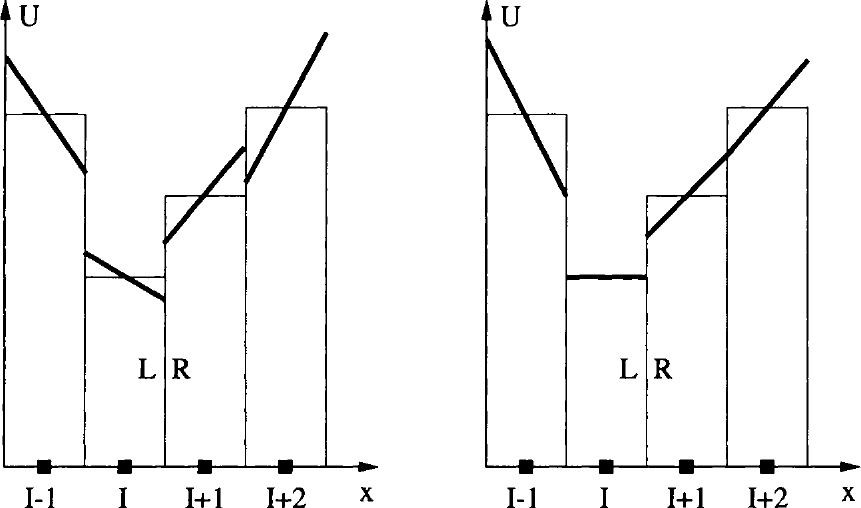
图4.11:向单元面直接插值(左)与限制插值(右)的比较。图例:粗线表示斜率\(\Delta U/\Delta x\)ï¼竖条表示单元中心处的值;横轴为\(I-1\)、\(I\)、\(I+1\)、\(I+2\)与\(x\),L、R标记面上的左、右状态。
下面我们描述四种业已确立并经实践检验的限制器函数:分别针对二阶MUSCL、CUSP以及上风TVD格式。en
In the following, we shall describe four different limiter functions, which are well-established and proven in practice. We shall consider limiters for the second-order MUSCL, for the CUSP and for the upwind TVD scheme.
Limiter Functions for MUSCL Interpolation 用于MUSCL插值的限制器函数
Van Leer的MUSCL方法[29]通过在必要时用限制器函数缩小方程(4.47)中的差分\(\Delta_{+}U_I\)与\(\Delta_{-}U_I\)ï¼即可成为保持单调性的格式。引入斜率限制器(slope limiter)\(\Phi^{\pm}\)后ï¼方程(4.46)中的MUSCL插值公式修改如下(另见图4.8)en
Van Leer's MUSCL approach [29] is turned into a monotonicity preserving scheme by employing a limiter function to reduce the differences \(\Delta_{+}U_I\) and \(\Delta_{-}U_I\) in Eq. (4.47) when necessary. Introducing slope limiters \(\Phi^{\pm}\), the MUSCL interpolation formulae in Eq. (4.46) are modified as follows (see also Fig. 4.8)
方程(4.46)中的参数\(\epsilon\)取为1。斜率限制器是相邻解变分之比的函数ï¼即\(\Phi^{\pm}_{I+1/2} = \Phi(r^{\pm}_{I+1/2})\)ï¼其定义[1]为en
The parameter \(\epsilon\) in Eq. (4.46) was set equal to unity. The slope limiters are functions of the ratios of the consecutive solution variations, i.e., \(\Phi^{\pm}_{I+1/2} = \Phi(r^{\pm}_{I+1/2})\), with the definitions [1]
若现在以\(r_L\)替代\(r^{+}_{I-1/2}\)、以\(r_R\)替代\(r^{-}_{I+3/2}\)ï¼即en
If we substitute now \(r_L\) for \(r^{+}_{I-1/2}\) and \(r_R\) for \(r^{-}_{I+3/2}\), thus
其中限制器函数(limiter function)定义为en
with the limiter function defined as
方程(4.110)中斜率限制器\(\Phi\)现在可以有不同的表述ï¼可针对特定的\(\hat{\kappa}\)值加以定制ï¼以得到最精确同时稳定且保持单调性的MUSCL格式。en
Different formulations of the slope limiter \(\Phi\) in Eq. (4.110) are now possible, which can be tailored to specific values of \(\hat{\kappa}\) to give the most accurate but stable and monotonicity preserving MUSCL scheme.
MUSCL scheme with \(\hat{\kappa}\) = 0 \(\hat{\kappa}\)=0的MUSCL格式
对\(\hat{\kappa} = 0\)的二阶上风偏置格式ï¼一种特别合适的组合是[92]en
One particularly suitable combination for the second-order, upwind-biased scheme with \(\hat{\kappa} = 0\) is [92]
此时ï¼函数\(\Psi(r)\)对应于Van Albada限制器[93]en
In this case, the function \(\Psi(r)\) corresponds to the Van Albada limiter [93]
函数\(\delta\)对两种状态在形式上完全相同ï¼即en
The function \(\delta\) is formally identical for both states. It reads
系数\(a\)与\(b\)对左、右状态定义为en
The coefficients \(a\) and \(b\) are defined for the left and right state as
差分算子\(\Delta_{\pm}\)由方程(4.47)给出。方程(4.114)中的附加参数\(\epsilon\)防止限制器在流动光滑区域因小尺度振荡而被激活[92];为获得完全收敛的定常解ï¼有时需要这样做。参数\(\epsilon\)宜取为与当地网格尺度成比例ï¼例如三维中取\(\Omega^{1/3}\)[92]、[94]。若状态变量\(U\)以物理单位给出ï¼则参数\(\epsilon\)还需附加缩放。可以证明ï¼对光滑变化的流动ï¼方程(4.113)的关系式与\(\hat{\kappa} = 0\)的原始(无限制)MUSCL格式(4.46)完全相同ï¼因此解的精度不受影响;另一方面ï¼函数\(\delta\)在局部极值处变为零ï¼如所期望地把精度降为一阶。en
and the difference operators \(\Delta_{\pm}\) are given by Eq. (4.47). The additional parameter \(\epsilon\) in Eq. (4.114) prevents the activation of the limiter in smooth flow regions due to small-scale oscillations [92]. This is sometimes necessary in order to achieve a fully converged steady-state solution. The parameter \(\epsilon\) is conveniently set proportional to the local grid scale, in 3D for example to \(\Omega^{1/3}\) [92], [94]. Additional scaling of the parameter \(\epsilon\) is required if the particular state variable \(U\) is given in physical units. It can be shown that the relations in Eq. (4.113) are identical to the original (unlimited) MUSCL scheme (4.46) with \(\hat{\kappa} = 0\) for smoothly varying flow. Thus, the accuracy of the solution is not influenced. On the other hand, the function \(\delta\) becomes zero at local extrema, reducing the accuracy to first order as desired.
MUSCL scheme with \(\hat{\kappa}\) = 1/3 \(\hat{\kappa}\)=1/3的MUSCL格式
针对\(\hat{\kappa} = 1/3\)的三点二阶精度上风偏置MUSCL格式ï¼设计了另一种限制器函数。此时斜率限制器为en
Another limiter function was devised for the three-point, second-order accurate upwind-biased MUSCL scheme with \(\hat{\kappa} = 1/3\). Here, the slope limiter is given by
此时ï¼函数\(\Psi(r)\)对应于Hemker与Koren的限制器[95]。按照与前一种情形相同的步骤ï¼得到的面\((I+1/2)\)处左、右状态公式与方程(4.113)相同ï¼只是\(\delta\)改为[92]en
In this case, the function \(\Psi(r)\) corresponds to the limiter of Hemker and Koren [95]. Following the same way as in the previous case, we obtain formulae for the left and right state at the face \((I+1/2)\) which are identical to Eq. (4.113), but now with [92]
系数\(a\)、\(b\)以及参数\(\epsilon\)的定义保持不变。en
The definitions of the coefficients \(a\), \(b\), and of the parameter \(\epsilon\) are retained.
Limiter for CUSP Scheme CUSP格式的限制器
在CUSP格式(4.3.2小节)框架下ï¼左(\(L\))、右(\(R\))状态按[43]以二阶精度计算en
In the framework of the CUSP scheme (Subsection 4.3.2), the left (\(L\)) and right (\(R\)) states are evaluated to second-order accuracy according to [43]
其中en
where
限制器本身定义为en
respectively. The limiter itself is defined as
其中\(\sigma\)为正常系数ï¼通常取2。常数\(\epsilon\)用于防止除零(例如\(\epsilon = 10^{-20}\))。若\(\Delta_1\)与\(\Delta_2\)恰好符号相反、大小相同ï¼则限制器变为\(\Psi = 0\)ï¼这意味着左、右状态只能得到一阶精度近似。en
where \(\sigma\) is a positive coefficient which is usually set equal to two. The constant \(\epsilon\) is required to prevent division by zero (e.g., \(\epsilon = 10^{-20}\)). If \(\Delta_1\) and \(\Delta_2\) happen to have opposite sign but the same magnitude, the limiter becomes \(\Psi = 0\). This means that we obtain only a first-order accurate approximation for the left and the right state.
应当指出ï¼也可以不用上述关系ï¼而代之以\(\hat{\kappa} = 0\)并采用方程(4.113)-(4.115)中Van Albada限制器的MUSCL格式。en
It should be mentioned that it is also possible to employ the MUSCL scheme with \(\hat{\kappa} = 0\) and the Van Albada limiter from Eqs. (4.113)-(4.115) instead of the above relations.
Limiter for TVD Scheme TVD格式的限制器
与前几种情形相比ï¼这里的限制器不作用于守恒变量或原始变量ï¼而是作用于特征变量\(\vec{C}\)。一种特别合适的限制器函数由[84]给出en
In comparison to the previous cases, the limiter here acts not on the conservative or the primitive variables, but on the characteristic variables \(\vec{C}\). One particularly suitable limiter function is given by [84]
其中\(\Delta C^{l}_{I+1/2}\)表示控制体面\((I+1/2)\)处特征变量之差(方程(4.101))。分母中的正常数\(\epsilon \approx 10^{-20}\)防止除零。在高梯度区域ï¼限制器函数变为零ï¼由方程(4.99)与方程(4.98)导致一阶精度的上风格式。当流动变量光滑变化时ï¼方程(4.98)的上风TVD格式保持二阶精度ï¼此时\(\Psi^{l}_{I} = C^{l}_{I} - C^{l}_{I-1}\)。en
where the \(\Delta C^{l}_{I+1/2}\) represents the difference of the characteristic variables at face \((I+1/2)\) of the control volume (Eq. (4.101)). The positive constant \(\epsilon \approx 10^{-20}\) in the denominator prevents division by zero. In regions with high gradients, the limiter function becomes zero, which leads with Eq. (4.99) and Eq. (4.98) to first-order accurate upwind scheme. The upwind TVD scheme in Eq. (4.98) retains second-order accuracy in areas with smoothly varying flow variables, where \(\Psi^{l}_{I} = C^{l}_{I} - C^{l}_{I-1}\).