chapter. Temporal Discretisation 第6章 时间离散[cfd-0007]
应用线方法(method of lines)ï¼即对控制方程(2.19)在空间和时间上分别进行离散化ï¼并对每个控制体写出来ï¼便得到一个时间上相互耦合的常微分方程组en
The application of the method of lines, i.e., the separate spatial and temporal discretisation of the governing equations (2.19), leads, written down for each control volume, to a system of coupled ordinary differential equations in time
在方程(6.1)中,\(\Omega\)表示体积,\(\vec{R}\)为残差,\(\bar{M}\)为质量矩阵ï¼下标\(I\)指某个具体的控制体。方程组(6.1)必须在时间上积分——或者为了得到定常解(\(\vec{R}_I = 0\))ï¼或者为了重现非定常流动的时间历程。en
In Eq. (6.1), \(\Omega\) represents the volume, \(\vec{R}\) the residual, \(\bar{M}\) the mass matrix, and the index \(I\) denotes the particular control volume. The system (6.1) has to be integrated in time - either to obtain a steady-state solution (\(\vec{R}_I = 0\)), or to reproduce the time history of an unsteady flow.
我们在3.2节简要讨论过方程组(6.1)求解的若干问题。我们看到ï¼各种显式(explicit)和隐式(implicit)方法都可以从一个基本的非线性格式导出。对静止网格ï¼该格式为en
We briefly discussed the aspects of the solution of the equation system (6.1) in Section 3.2. We saw that the various explicit and implicit methods can be derived from a basic non-linear scheme. It reads for a stationary grid
其中en
where
表示解的更新(updateï¼即修正量)。上标\(n\)和\((n+1)\)表示时间层。因此,\(\vec{W}^n\)指当前时刻\(t\)的流动解ï¼而\(\vec{W}^{n+1}\)表示时刻\((t+\Delta t)\)的解。参数\(\beta\)和\(\omega\)决定离散化类型(显式或隐式)ï¼也决定时间精度。例如ï¼要达到二阶时间精度ï¼必须满足方程(3.6)所表达的条件。en
stands for the update (correction) of the solution. The superscripts \(n\) and \((n+1)\) denote the time levels. Hence, \(\vec{W}^n\) means the flow solution at the present time \(t\). Consequently, \(\vec{W}^{n+1}\) represents the solution at the time \((t+\Delta t)\). The parameters \(\beta\) and \(\omega\) determine the discretisation type (explicit or implicit) and also the temporal accuracy. For example, the condition expressed by Eq. (3.6) must be fulfilled to achieve second-order temporal accuracy.
在下面几节中ï¼我们将较为详细地讨论最常用的显式和隐式时间推进方法。我们还将说明如何针对具体格式计算最大允许时间步长。此外ï¼我们还要讨论在结构网格和非结构网格上的恰当实现问题。最后ï¼本章末节将专门讨论非定常流动问题的时间精确解。en
In the following sections, we shall consider the most popular explicit and implicit time-stepping methods in some detail. We shall also present how the maximum allowable time step can be evaluated for a particular scheme. Furthermore, we shall discuss the issues of the appropriate implementations on structured as well as on unstructured grids. Finally, the last section will be devoted to time-accurate solutions of unsteady flow problems.
6.1 Explicit Time-Stepping Schemes 显式时间推进格式[cfd-6-1]
显式格式从已知解\(\vec{W}^n\)出发ï¼利用相应的残差\(\vec{R}^n\)来得到时刻\((t+\Delta t)\)的新解。换言之ï¼新解\(\vec{W}^{n+1}\)只依赖于已经已知的值。这一事实使显式格式非常简单、易于实现。en
An explicit scheme starts from a known solution \(\vec{W}^n\) and employs the corresponding residual \(\vec{R}^n\) in order to obtain a new solution at time \((t+\Delta t)\). In other words, the new solution \(\vec{W}^{n+1}\) depends solely on values already known. This fact makes the explicit schemes very simple and easy to implement.
该式称为前向Euler(forward Euler)近似。对于定常问题或单元中心离散化ï¼质量矩阵\(\bar{M}\)可以集中(lumpedï¼即用单位矩阵代替)。en
which is termed the forward Euler approximation. The mass matrix \(\bar{M}\) can be lumped (i.e., substituted by the identity matrix) for steady problems or for the cell-centred discretisation.
目前最流行、应用最广的显式方法是多步(multistage,Runge-Kutta)时间推进格式及其变体——混合(hybrid)多步格式。因此ï¼下面我们将介绍这两种方法。en
The by far most popular and widespread explicit method is the multistage (Runge-Kutta) time-stepping scheme and its variant the hybrid multistage scheme. Therefore, we shall describe both methods below.
6.1.1 Multistage Schemes (Runge-Kutta) 多步格式(Runge-Kutta)[cfd-6-1-1]
显式多步格式的概念最早由Jameson等人[1]提出。多步格式通过若干步——所谓阶段(stages)——来推进解ï¼每一步都可以看作按方程(6.4)进行的一次更新。将其应用于质量矩阵已集中的离散化控制方程(6.1),\(m\)步(m-stage)格式为en
The concept of explicit multistage schemes was first presented by Jameson et al. [1]. The multistage scheme advances the solution in a number of steps - so-called stages - which can be viewed as a sequence of updates according to Eq. (6.4). Applied to the discretised governing equations (6.1), where the mass matrix was lumped, an \(m\)-stage scheme reads
在上面的表达式(6.5)中,\(\alpha_k\)表示阶段系数。此外ï¼记号\(\vec{R}_I^{(k)}\)表示残差用第\(k\)步的解\(\vec{W}_I^{(k)}\)来求值。en
In the above expressions (6.5), \(\alpha_k\) represents the stage coefficients. Furthermore, the denotation \(\vec{R}_I^{(k)}\) means that the residual is evaluated with the solution \(\vec{W}_I^{(k)}\) from the \(k\)-th stage.
与经典Runge-Kutta格式不同ï¼这里为了减少内存需求ï¼只存储第零步的解和最新的残差。针对具体的空间离散化ï¼可以调整阶段系数ï¼以增大最大时间步长并改善稳定性[2]-[4]。为保持一致性ï¼只要求\(\alpha_m = 1\)。对Runge-Kutta格式作这一修改的后果是:只有当\(\alpha_{m-1} = 1/2\)时才能实现二阶时间精度;否则ï¼多步格式在时间上只有一阶精度。en
Unlike in the classical Runge-Kutta schemes, only the zeroth solution and the newest residual are stored here in order to reduce the memory requirements. The stage coefficients can be tuned to increase the maximum time step and to improve the stability for a particular spatial discretisation [2]-[4]. For consistency, it is only required that \(\alpha_m = 1\). A consequence of the modification to the Runge-Kutta scheme is that second-order time accuracy can be realised only if \(\alpha_{m-1} = 1/2\). Otherwise, the multistage scheme is first-order accurate in time.
上述多步方法(6.5)特别适合于结构网格和非结构网格上的上风空间离散化。中心离散化格式与下面要介绍的混合多步方法配合使用则效率更高。表6.1给出一阶和二阶上风格式在3步至5步格式下的优化阶段系数[2]。实践经验表明ï¼当流场中含有强激波时ï¼无论空间离散化的阶数如何ï¼都应优先选用一阶格式的系数。这可以解释为:任何高阶格式都会在激波处降为一阶ï¼以防止解的振荡;而强激波处的残差对收敛到定态的影响最为显著。en
The above multistage approach (6.5) is particularly suitable for upwind spatial discretisation on structured as well as unstructured grids. Central discretisation schemes perform more efficiently with the hybrid multistage methodology, which will be described next. Sets of optimised stage coefficients for first- and second-order upwind schemes are presented in Table 6.1 for three- to five-stage schemes [2]. Practical experience shows that the coefficients for the first-order scheme should be preferred in cases, where the flow field contains strong shocks, regardless of the order of the spatial discretisation. This can be explained by the fact that every higher-order scheme switches to first order at shocks to prevent oscillations of the solution. However, the residuals at strong shocks influence the convergence to steady state most significantly.
(见原书第185页 表6.1ï¼多步格式:一阶与二阶上风空间离散化的优化阶段系数(α)与CFL数(σ))
          first-order scheme       second-order scheme
stages  3      4      5       3      4      5
sigma   1.5    2.0    2.5     0.69   0.92   1.15
alpha_1 0.1481 0.0833 0.0533  0.1918 0.1084 0.0695
alpha_2 0.4000 0.2069 0.1263  0.4929 0.2602 0.1602
alpha_3 1.0000 0.4265 0.2375  1.0000 0.5052 0.2898
alpha_4        1.0000 0.4414         1.0000 0.5060
alpha_5               1.0000                1.0000
表6.1:多步格式:一阶与二阶上风空间离散化的优化阶段系数(α)与CFL数(σ)。
(见原书第185页 表6.2ï¼混合多步格式:中心格式与上风空间离散化的优化阶段系数(α)、混合系数(β)及CFL数(σ))
         central scheme    1st-order upwind   2nd-order upwind
         sigma = 3.6       sigma = 2.0        sigma = 1.0
stage    alpha   beta      alpha   beta       alpha   beta
1        0.2500  1.00      0.2742  1.00       0.2742  1.00
2        0.1667  0.00      0.2067  0.00       0.2067  0.00
3        0.3750  0.56      0.5020  0.56       0.5020  0.56
4        0.5000  0.00      0.5142  0.00       0.5142  0.00
5        1.0000  0.44      1.0000  0.44       1.0000  0.44
表6.2:混合多步格式:中心格式与上风空间离散化的优化阶段系数(α)、混合系数(β)及CFL数(σ)。注意:一阶与二阶上风格式的系数完全相同ï¼但CFL数不同。
一切显式格式的主要缺点是:时间步长(\(\Delta t\))受到控制方程的特征以及网格几何的严格限制。我们将在6.1.4小节讨论最大允许时间步长的计算。时间步长和所谓CFL数(CFL number)确定的理论问题将在10.3节稳定性分析中考察。en
The main disadvantage of every explicit scheme is that the time step (\(\Delta t\)) is severely restricted by the characteristics of the governing equations as well as by the grid geometry. We shall discuss the computation of the maximum allowable time step in Subsection 6.1.4. Theoretical aspects of the determination of the time step and the so-called CFL number will be considered in Section 10.3 on stability analysis.
6.1.2 Hybrid Multistage Schemes 混合多步格式[cfd-6-1-2]
把显式多步格式(6.5)应用于方程组(6.1)时ï¼如果黏性通量和耗散不在每个阶段都重新求值ï¼计算量可以大幅减少。此外ï¼还可以把不同阶段的耗散项混合(blend)起来ï¼以提高格式的稳定性。这类方法由Martinelli[5]和Mavriplis等人[6]提出ï¼称为混合多步格式(hybrid multistage schemes)。只要阶段系数经过仔细优化ï¼混合格式与基本多步格式一样稳健。en
The computational work of an explicit multistage scheme (6.5), applied to the system (6.1), can be substantially reduced if the viscous fluxes and the dissipation are not re-evaluated at each stage. Additionally, the dissipation terms from different stages can be blended to increase the stability of the scheme. Methods of this type were devised by Martinelli [5] and by Mavriplis et al. [6]. They are known as hybrid multistage schemes. Provided the stage coefficients are carefully optimised, the hybrid schemes are as robust as the basic multistage schemes.
为便于说明ï¼考虑一种常用的5步混合格式ï¼其耗散项只在奇数步求值——一般记为(5,3)格式。首先ï¼把空间离散化分成两部分ï¼即en
Let us for illustration consider a popular 5-stage hybrid scheme, where the dissipative terms are evaluated at odd stages - generally denoted as the (5,3)-scheme. First, we split the spatial discretisation into two parts, i.e.,
第一部分\(\vec{R}_c\)包含对流通量的中心离散化——可以是变量平均ï¼也可以是通量平均——还包括源项。第二部分\(\vec{R}_d\)由黏性通量和数值耗散组成。例如ï¼对于带人工耗散的中心格式(4.3.1或5.3.1小节)ï¼可取en
The first part, \(\vec{R}_c\), contains the central discretisation of the convective fluxes, which can be either the average of variables or the average of fluxes. It also includes the source term. The second part, \(\vec{R}_d\), is composed of the viscous fluxes and the numerical dissipation. For example, in the case of the central scheme with artificial dissipation (Subsections 4.3.1 or 5.3.1) we would set
其中\(\vec{W}_{av}\)表示面\(k\)左右两侧流动变量的算术平均。en
where \(\vec{W}_{av}\) represents the arithmetic average of flow variables from the left and the right side of face \(k\).
其中en
where
上述关系(6.7)、(6.8)中的阶段系数\(\alpha_m\)和混合系数\(\beta_m\)在表6.2中针对中心格式和上风格式给出。这两组系数都是专门针对多重网格方法(9.4节)优化的。上述混合多步格式的性质将在10.3节中讨论。en
The stage coefficients \(\alpha_m\) and the blending coefficients \(\beta_m\) in the above relations (6.7), (6.8) are given in Table 6.2 for central and upwind schemes. Both sets of coefficients are particularly optimised for the multigrid method (Section 9.4). We shall discuss the properties of the above hybrid multistage scheme later in Section 10.3.
应当指出ï¼另一种常见的做法是只在头两步求值耗散项\(\vec{R}_d\)ï¼而不做任何混合。著名的(5,2)格式常与中心空间离散化配合使用ï¼它采用表6.2中的阶段系数。然而ï¼与上述(5,3)格式相比,(5,2)格式不太适合黏性流动和多重网格。en
It should be mentioned that it is also popular to evaluate the dissipation term \(\vec{R}_d\) in the first two stages only, without any blending. A well-known (5,2)-scheme, which is often employed with the central spatial discretisation, uses the stage coefficients of Table 6.2. However, the (5,2)-scheme is less suitable for viscous flows and multigrid than the above (5,3)-scheme.
6.1.3 Treatment of the Source Term 源项的处理[cfd-6-1-3]
在某些情形下ï¼方程(4.2)或(5.2)中的源项\(\vec{Q}\)会变得占主导地位。采用化学或湍流模型时经常会遇到这种情况。问题在于ï¼大的源项会使流动变量在空间和时间上迅速变化。强源项引起的变化发生在比流动方程的时间尺度小得多的时间尺度上。这会显著增大控制方程的刚性(stiffness)。刚性定义为雅可比矩阵\(\partial\vec{R}/\partial\vec{W}\)的最大特征值与最小特征值之比。刚性也可以看作最大时间尺度与最小时间尺度之比。en
There are certain cases in which the source term \(\vec{Q}\) in Eq. (4.2) or (5.2) becomes dominant. Such situation is often encountered when chemistry or turbulence models are employed. The problem is that a large source term changes the flow variables rapidly in space and in time. The changes due to a strong source term happen at much smaller time scales than those of the flow equations. This increases the stiffness of the governing equations significantly. The stiffness is defined as the ratio of the largest to the smallest eigenvalue of the Jacobian matrix \(\partial\vec{R}/\partial\vec{W}\). The stiffness can also be viewed as the ratio of the largest to the smallest time scale.
把上述显式多步格式(或任何其他纯显式格式)应用于刚性方程组时ï¼为使时间积分稳定ï¼必须大幅减小时间步长ï¼于是向定态的收敛会变得非常慢。更严重的是ï¼显式格式甚至可能找不到正确的解[7]。Curtiss等人[8]提出的补救办法是以隐式方式处理源项。为演示这一方法ï¼把方程(6.4)的基本显式格式改写如下(参见方程(4.2)或(5.2))en
When we apply one of the above explicit multistage schemes (or any other purely explicit scheme) to a stiff system of equations, we will have to reduce the time step considerably in order to stabilise the time integration. Hence, the convergence to the steady state will become very slow. More seriously, an explicit scheme can even fail to find the correct solution [7]. A remedy suggested by Curtiss et al. [8] is to treat the source term in an implicit way. In order to demonstrate the approach, we rewrite the basic explicit scheme in Eq. (6.4) as follows (cf. Eq. (4.2) or (5.2))
其中源项现在在新时间层\((n+1)\)处求值。为简单起见ï¼方程(6.9)中略去了质量矩阵。由于时刻\((n+1)\)的源项值未知ï¼必须对它作近似。为此ï¼把源项在当前时间层\(n\)处线性化ï¼得到en
where the source term is now evaluated at the new time level \((n+1)\). For simplicity, the mass matrix was omitted from Eq. (6.9). Since the value of the source term at the time \((n+1)\) is unknown, we have to approximate it. For this purpose, we linearise the source term about the current time level \(n\), resulting in
其中\(\bar{I}\)表示单位矩阵。式(6.11)称为点隐式(point implicit)ï¼因为左端方括号内的项——即隐式算子——只依赖控制体\(\Omega_I\)自身的值。与方程(6.9)比较可知ï¼标量时间步长\(\Delta t\)现在变成了一个矩阵。这样ï¼每个流动方程都被一个单独的参数(对应于相应的特征值)所缩放。如此一来ï¼时间尺度之间的差异得到补偿ï¼源项造成的时间步长限制得以缓解。en
where \(\bar{I}\) represents the identity matrix. The formulation (6.11) is called point implicit because the term in square brackets on the left-hand side - the implicit operator - depends only on values in the control volume \(\Omega_I\) itself. A comparison with Eq. (6.9) reveals that the scalar time step \(\Delta t\) changed now to a matrix. Thus, each flow equation becomes scaled by an individual parameter, corresponding to the associated eigenvalue. In this way, the disparity between the time scales is offset and the time step restriction due to the source term is alleviated.
更精细的做法是用半隐式Runge-Kutta格式来处理刚性源项ï¼该格式最早由Rosenbrock[14]提出。这种格式在数值上比方程(6.12)的方法更稳定ï¼但要求在每个阶段对一个大型线性方程组求逆。半隐式Runge-Kutta格式的细节及应用可参见文献[15]-[18]。en
A more elaborate approach is to treat the stiff source term by means of an semi-implicit Runge-Kutta scheme, originally suggested by Rosenbrock [14]. The scheme is numerically more stable than the approach in Eq. (6.12), however it requires the inversion of a large system of linear equations at each stage. Details of the semi-implicit Runge-Kutta scheme and applications can be found in Refs. [15]-[18].
6.1.4 Determination of the Maximum Time Step 最大时间步长的确定[cfd-6-1-4]
每一种显式时间推进格式都只在时间步长\(\Delta t\)不超过某个值时才保持稳定。为使格式稳定ï¼时间推进格式必须满足所谓的Courant-Friedrichs-Lewy(CFL)条件[19]。该条件指出:数值方法的依赖域必须包含偏微分方程的依赖域。对基本显式格式(6.4)而言,CFL条件意味着时间步长应等于或小于信息越过空间离散化格式模板(stencil)所需的时间。因此ï¼对一维线性对流方程ï¼时间步长条件为en
Every explicit time-stepping scheme remains stable only up to a certain value of the time step \(\Delta t\). To be stable, a time-stepping scheme has to fulfil the so-called Courant-Friedrichs-Lewy (CFL) condition [19]. It states that the domain of dependence of the numerical method has to include the domain of dependence of the partial differential equation. The CFL condition means for the basic explicit scheme (6.4) that the time step should be equal to or smaller than the time required to transport information across the stencil of the spatial discretisation scheme. Hence, in 1D the condition for the time step would read for the linear convection equation
其中\(\Delta x/|\Lambda_c|\)表示以速度\(\Lambda_c\)把信息传播过一个单元尺寸\(\Delta x\)所需的时间。速度\(\Lambda_c\)对应于对流通量雅可比的最大特征值。正常数\(\sigma\)表示CFL数(CFL number)。CFL数的大小取决于时间推进格式的类型和参数ï¼也取决于空间离散化格式的形式。我们将在10.3节中针对两个模型问题研究\(\sigma\)的依赖关系。表6.1和表6.2列出了各种多步格式和离散化的CFL数。en
where \(\Delta x/|\Lambda_c|\) represents the time necessary to propagate information over the cell size \(\Delta x\) with the velocity \(\Lambda_c\). The velocity \(\Lambda_c\) corresponds to the maximum eigenvalue of the convective flux Jacobian. The positive coefficient \(\sigma\) denotes the CFL number. The magnitude of the CFL number depends on the type and the parameters of the time-stepping scheme, as well as on the form of the spatial discretisation scheme. We shall investigate the dependency of \(\sigma\) in Section 10.3 for two model problems. Tables 6.1 and 6.2 list the CFL numbers for various multistage schemes and discretisations.
对于线性模型方程ï¼可以借助Von Neumann稳定性分析(10.3节)确定最大时间步长。然而ï¼在多维情形和非线性控制方程下ï¼最大时间步长只能近似计算。下面我们将给出在结构网格和非结构网格上、对无黏和黏性流动估计时间步长的关系式。en
The maximum time step can be determined for linear model equations with the aid of Von Neumann stability analysis (Section 10.3). However, the maximum time step can be calculated only approximately in multiple dimensions and for non-linear governing equations. In the following, we will present relations for the estimation of the time step on structured and unstructured grids, and for inviscid as well as for viscous flows.
Time Step on Structured Grids 结构网格上的时间步长
Euler Equations 欧拉方程
在结构网格上ï¼对控制体\(\Omega_I\)ï¼时间步长\(\Delta t\)可以由近似关系[20]-[22]确定en
On a structured grid, the time step \(\Delta t\) can be determined for a control volume \(\Omega_I\) from the approximate relation [20]-[22]
CFL数\(\sigma\)对多步格式在表6.1中给出ï¼对混合格式在表6.2中给出。对流通量雅可比(A.9)的谱半径对三个网格方向分别为en
The CFL number \(\sigma\) is given for multistage schemes in Table 6.1 and for hybrid schemes in Table 6.2. The spectral radii of the convective flux Jacobians (A.9) read for the three grid directions
方程(6.15)中的法向量和面面积ï¼由相应方向上控制体两个相对侧面处的对应值平均得到。例如ï¼若对偶控制体(4.2.3小节)的取向如图4.1b所示ï¼则在\(I\)方向上应取en
The normal vectors and face areas in Eq. (6.15) are obtained by averaging the corresponding values from the two opposite sides of the control volume in the respective direction. For example, if a dual control volume (Subsection 4.2.3) would be oriented as sketched in Fig. 4.1b, we would use in the \(I\)-direction
\(J\)方向和\(K\)方向也有类似的表达式。用方程(6.14)得到的是局部(local)时间步ï¼它只对一个控制体有效。如果我们要求定常解ï¼可以用局部时间步来加速收敛(参见9.1节)。但如果时间精度重要ï¼就必须对所有控制体采用同一个全局(global)时间步ï¼即en
Similar expressions hold for the \(J\)- and \(K\)-direction. With Eq. (6.14), we obtain a local time step, which is valid for one control volume only. If we are interested in a steady state solution, we may use the local time step to accelerate the convergence (cf. Section 9.1). However, if time accuracy is important, we have to employ one global time step for all volumes, i.e.,
即对所有控制体取最小值。en
where the minimum over all control volumes is taken.
Navier-Stokes Equations Navier-Stokes方程
对黏性流动ï¼计算\(\Delta t\)时还必须计入黏性通量雅可比(A.10)的谱半径。在边界层内ï¼它们可能严重限制最大时间步长。时间步长可由下式计算[5]、[21]、[22]en
For viscous flows, the spectral radii of the viscous flux Jacobians (A.10) have to be included in the computation of \(\Delta t\). They can severely limit the maximum time step in boundary layers. The time step can be evaluated from [5], [21], [22]
乘在黏性谱半径上的常数ï¼对中心空间离散化通常取\(C = 4\)ï¼一阶上风离散化取\(C = 2\)ï¼二阶上风离散化取\(C = 1\)。若假定采用涡黏性湍流模型ï¼则黏性谱半径由下式给出[21]、[22]en
The constant which multiplies the viscous spectral radii is usually set as \(C = 4\) for central spatial discretisations, \(C = 2\) for first-order upwind and \(C = 1\) for second-order upwind discretisations. If we assume that an eddy-viscosity turbulence model is employed, the viscous spectral radii are given by [21], [22]
其他方向与此类似。方程(6.19)中,\(\mu_L\)和\(\mu_T\)分别表示层流和湍流的动力黏度系数;\(Pr_L\)和\(Pr_T\)为层流和湍流Prandtl数。表6.1和表6.2中的CFL数也适用于黏性流动。对黏性流动特别有效的是方程(6.7)的(5,3)混合格式。en
and similarly for the other directions. In Equation (6.19), \(\mu_L\) denotes the laminar and \(\mu_T\) the turbulent dynamic viscosity coefficient, respectively. Furthermore, \(Pr_L\) and \(Pr_T\) are the laminar and the turbulent Prandtl numbers. The CFL numbers in Tables 6.1 and 6.2 apply also for viscous flows. Particularly efficient for viscous flows is the (5,3) hybrid scheme from Eq. (6.7).
Time Step on Unstructured Grids 非结构网格上的时间步长
已经提出了若干种在非结构网格上估计最大时间步长的方法。下面介绍两种不同的方法。en
Several approaches were suggested for the estimation of the maximum time step on unstructured grids. We shall present two different approaches below.
Method 1 方法1
一种经过验证、与结构网格上的实现非常接近的方法为[6]en
One proven method, which closely follows the implementation on structured grids, reads [6]
其中\(\hat{\Lambda}_c\)和\(\hat{\Lambda}_v\)表示控制体所有面上对流谱半径和黏性谱半径之和。与结构网格上一样ï¼通常取\(1 \le C \le 4\)。对单元中心格式ï¼谱半径定义为[6]en
where \(\hat{\Lambda}_c\) and \(\hat{\Lambda}_v\) represent a sum of the convective and viscous spectral radii over all faces of the control volume. As on structured grids, \(1 \le C \le 4\) is usually used. In the case of the cell-centred scheme, the spectral radii are defined as [6]
控制体各面上的流动变量之值由算术平均得到。en
The values of the flow variables at the faces of the control volume are obtained by arithmetic averaging.
Method 2 方法2
方程(6.21)预测的谱半径偏大ï¼在混合单元网格上尤其如此。这导致时间步长小于稳定所需的值。文献[23]中的实现提供了对时间步长更准确的估计ï¼即en
The spectral radii predicted by Eq. (6.21) are too large, particularly on mixed element grids. This leads to a smaller time step than required for the stability. The implementation in Ref. [23] offers a more accurate estimation of the time step, namely
其中对流谱半径为en
with the convective spectral radii
黏性谱半径为(假定采用涡黏性湍流模型)en
and with the viscous spectral radii (eddy-viscosity turbulence model assumed)
变量\(\Delta\hat{S}^x\)、\(\Delta\hat{S}^y\)和\(\Delta\hat{S}^z\)分别表示控制体在\(y\)-\(z\)、\(x\)-\(z\)和\(x\)-\(y\)平面上的投影。它们由下列公式给出en
The variables \(\Delta\hat{S}^x\), \(\Delta\hat{S}^y\) and \(\Delta\hat{S}^z\), respectively, represent projections of the control volume on the \(y\)-\(z\)-, \(x\)-\(z\)- and the \(x\)-\(y\)-plane. They are given by the formulae
其中\(S_x\)、\(S_y\)和\(S_z\)表示面向量\(\vec{S} = \vec{n}\cdot\Delta S\)的\(x\)、\(y\)和\(z\)分量。CFL数一般与结构网格上的相同ï¼因此表6.1和表6.2中收集的数值仍然适用。此外ï¼向定态的收敛同样可以用局部时间推进来加速ï¼做法与结构网格上一样。模拟非定常流动所需的全局时间步ï¼与前面一样由方程(6.17)得到。en
where \(S_x\), \(S_y\) and \(S_z\) denote the \(x\)-, \(y\)- and the \(z\)-component of the face vector \(\vec{S} = \vec{n}\cdot\Delta S\). The CFL numbers stay in general the same as on structured grids. Thus, the values collected in Tables 6.1 and 6.2 still apply. Furthermore, the convergence to steady state can also be accelerated by local time stepping, in the same way as on the structured grids. A global time step, necessary for simulating unsteady flows, can be obtained from Eq. (6.17) as before.
6.2 Implicit Time-Stepping Schemes 隐式时间推进格式[cfd-6-2]
可以看出ï¼隐式形式导出一组关于时刻\((t+\Delta t)\)未知流动变量的非线性方程。求解方程(6.26)需要在新时间层上求值残差ï¼即\(\vec{R}^{n+1}\)。由于我们不知道\(\vec{W}^{n+1}\)ï¼这无法直接进行。不过ï¼可以把方程(6.26)中的残差\(\vec{R}^{n+1}\)在当前时间层处线性化ï¼即en
As we can see, the implicit formulation leads to a set of non-linear equations for the unknown flow variables at the time \((t+\Delta t)\). The solution of Eq. (6.26) requires the evaluation of the residual at the new time level, i.e., \(\vec{R}^{n+1}\). Since we do not know \(\vec{W}^{n+1}\), this cannot be done directly. However, we can linearise the residual \(\vec{R}^{n+1}\) in Eq. (6.26) about the current time level, i.e.,
其中\(\partial\vec{R}/\partial\vec{W}\)一项称为通量雅可比(flux Jacobian)。应当指出ï¼通量雅可比常常是由\(\vec{R}^n\)所表示的空间离散化的一个相当粗糙的近似导出的。例如ï¼对高阶上风离散化ï¼通常只基于一阶上风格式来构造通量雅可比。然而ï¼为了获得最佳效率和稳健性ï¼通量雅可比仍应反映空间离散化最重要的特征。en
where the term \(\partial\vec{R}/\partial\vec{W}\) is referred to as the flux Jacobian. We should mention that the flux Jacobian is often derived from a rather crude approximation to the spatial discretisation represented by \(\vec{R}^n\). For example, in the case of higher-order upwind discretisations, it is quite common to base the flux Jacobian solely on a first-order upwind scheme. However, for best efficiency and robustness, the flux Jacobian should still reflect the most important features of the spatial discretisation.
隐式算子构成一个大型、稀疏、非对称的块矩阵ï¼其维数等于单元总数(单元中心格式)或网格点总数(单元顶点格式)。下面我们将进一步讨论隐式算子在结构网格和非结构网格上的形式。如3.2节所述ï¼质量矩阵\(\bar{M}\)可以用单位矩阵代替ï¼而不影响定常解。方程(6.28)中的参数\(\beta\)一般取1ï¼这样得到一阶精度的时间离散化。\(\beta = 1/2\)时可以得到二阶时间精度格式ï¼但不推荐这样做ï¼因为\(\beta = 1\)的格式稳健得多ï¼而且对定常问题时间精度并不重要。en
The implicit operator constitutes a large, sparse, and non-symmetric block matrix with dimensions equal to the total number of cells (cell-centred scheme) or grid points (cell-vertex scheme). Below we will discuss further the form of the implicit operator for structured as well as for unstructured grids. As we already saw in Section 3.2, the mass matrix \(\bar{M}\) can be replaced by the identity matrix, without influencing the steady state solution. The parameter \(\beta\) in Eq. (6.28) is generally set to 1, which results in a 1st-order accurate temporal discretisation. A 2nd-order time accurate scheme is obtained for \(\beta = 1/2\). However, this is not recommended since the scheme with \(\beta = 1\) is much more robust, and the time accuracy is of no importance for steady problems.
当控制方程为刚性方程时ï¼必须把源项纳入隐式算子。方程(6.27)中残差的线性化十分自然地做到了这一点ï¼它给出的形式与方程(6.10)完全相同。如文献[12]所证明的ï¼只要\(\partial\vec{Q}/\partial\vec{W}\)的特征值全为负或零ï¼上述隐式格式(6.28)对任意时间步长都保持稳定。en
In the case of stiff governing equations, the source term has to be included in the implicit operator. This happens quite naturally with the linearisation of the residual in Eq. (6.27), which leads to a formulation identical to Eq. (6.10). As demonstrated in Ref. [12], the above implicit scheme (6.28) remains stable for any time step if the eigenvalues of \(\partial\vec{Q}/\partial\vec{W}\) are all negative or zero.
求解线性方程组(6.28)需要对隐式算子求逆ï¼即对一个非常大的矩阵求逆。原则上这有两种做法。第一种是直接矩阵求逆ï¼采用Gaussian消元或某种直接稀疏矩阵方法[24]、[25]。然而ï¼由于内存需求过大、计算量极高ï¼这一方法不适合实际问题[26]。en
The solution of the linear equation system (6.28) requires the inversion of the implicit operator, i.e., the inversion of a very large matrix. In principle, this can be done in two ways. The first one consists of a direct matrix inversion, using either the Gaussian elimination or some direct sparse matrix method [24], [25]. However, because of the excessive amount of memory and the very high computational effort, this approach is not suited for practical problems [26].
对隐式算子求逆的第二类方法是迭代方法。我们在3.2.2小节提到了使用最广的几种迭代方法。迭代方法大致可以分为两类。第一类是把隐式算子分解成若干部分的做法——这一过程称为因式分解(factorisation)。各因子的构造方式使其比原来的隐式算子更容易求逆。第二类是采用Krylov子空间方法求隐式算子之逆的格式。在这种情形下ï¼通常令\(\Delta t \rightarrow \infty\)ï¼把隐式时间推进格式(6.28)化为牛顿法ï¼这样的格式随即称为Newton-Krylov方法。en
The second possibility of inverting the implicit operator represent iterative methods. We mentioned the most widely used ones in Subsection 3.2.2. Iterative methods can be divided roughly into two groups. The first one consists of approaches which decompose the implicit operator into several parts - a process called factorisation. The factors are constructed in such a way that they can be more easily inverted than the original implicit operator. To the second group belong schemes, which employ a Krylov-subspace method for the inversion of the implicit operator. In this case, the implicit time-stepping scheme (6.28) is usually turned into Newton's method by setting \(\Delta t \rightarrow \infty\). The scheme is then named Newton-Krylov method.
下面我们先讨论隐式算子的矩阵结构ï¼然后研究计算方程(6.28)中通量雅可比\(\partial\vec{R}/\partial\vec{W}\)的各种途径ï¼最后详细介绍三种最常用的迭代方法。en
In the following, we shall discuss first the matrix structure of the implicit operator. Then, we shall investigate the possibilities of computing the flux Jacobian \(\partial\vec{R}/\partial\vec{W}\) in Eq. (6.28). Finally, we shall present the three most popular iterative methods in detail.
6.2.1 Matrix Form of the Implicit Operator 隐式算子的矩阵形式[cfd-6-2-1]
其中\(N_F\)为控制体\(\Omega\)的面数(参见方程(4.2)或(5.2))。于是ï¼通量雅可比为en
with \(N_F\) being the number of faces of the control volume \(\Omega\) (cf. Eq. (4.2) or (5.2)). Thus, the flux Jacobian reads
需要强调的是ï¼必须把通量雅可比理解为作用在更新量\(\Delta\vec{W}\)上的一个算子。如上所述ï¼方程(6.30)中的对流通量和黏性通量不一定非要与显式算子中的通量完全相同。en
It should be stressed that the flux Jacobian has to be conceived as an operator which acts on the update \(\Delta\vec{W}\). As stated above, the convective and viscous fluxes in Eq. (6.30) do not necessarily have to be identical to the fluxes in the explicit operator.
由于结构网格和非结构网格上的隐式算子差别很大ï¼我们将分别讨论这两种情形。en
Because of the significant differences between the implicit operators on structured and unstructured grids, we shall treat each case separately.
Implicit Operator on Structured Grids 结构网格上的隐式算子
为了导出方程(6.28)中系统矩阵的形式ï¼考察图6.1所示的一维网格。进一步假设空间离散化采用带对偶控制体的单元顶点格式(4.2.3小节)和简单的通量平均(参见图4.8)。在没有黏性通量的情形下ï¼残差为en
In order to derive the form of the system matrix in Eq. (6.28), let us consider the 1-D grid in Fig. 6.1. Let us further assume that the cell-vertex scheme with dual control volumes (Subsection 4.2.3) and a simple average of fluxes are used for the spatial discretisation (cf. Fig. 4.8). In the absence of viscous fluxes, the residual is given by
其中\(\bar{I}\)代表单位矩阵。应当注意ï¼每个矩阵\(\bar{A}_c\)中的单位法向量都在与相应面积\(\Delta S\)相同的控制体一侧求值。可以看到ï¼隐式算子涉及与空间离散化相同的三点模板(节点\(i-1\)、\(i\)和\(i+1\))。en
where \(\bar{I}\) stands for the identity matrix. It should be noted that the unit normal vector in each matrix \(\bar{A}_c\) is evaluated at the same side of the control volume as the associated area \(\Delta S\). As we can see, the implicit operator involves the same 3-point stencil (nodes \(i-1\), \(i\), and \(i+1\)) as the spatial discretisation.
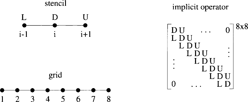
图6.1:一维结构网格及相应的三点模板隐式算子矩阵。图例:左上为模板(stencil)——节点\(L\)(\(i-1\))、\(D\)(\(i\))、\(U\)(\(i+1\));左下为网格(grid)——编号1至8的8个网格节点;右侧为隐式算子——\(8\times 8\)块三对角矩阵ï¼非零块为\(L\)、\(D\)、\(U\)ï¼角落处为0。
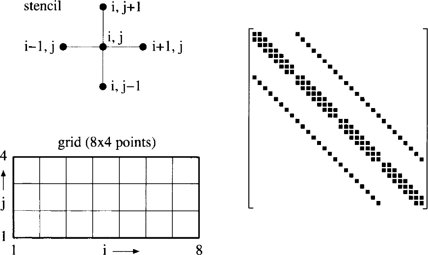
图6.2:二维结构网格(左)及相应的五点模板隐式算子矩阵(右)。图例:模板(stencil)由节点\(i,j\)及其四个邻居\(i-1,j\)、\(i+1,j\)、\(i,j-1\)、\(i,j+1\)组成;网格(grid)为\(8\times 4\)个节点,\(i\)方向编号1至8,\(j\)方向编号1至4;右侧矩阵中非零块矩阵以实心方块表示。
为了将系统矩阵可视化ï¼把隐式算子中与中心节点\(i\)相关联的所有项记为\(\mathbf{D}\)ï¼即en
In order to visualise the system matrix, we denote all terms in the implicit operator associated with the central node \(i\) as \(\mathbf{D}\), i.e.,
把下游节点\((i+1)\)记为\(\mathbf{U}\)ï¼即en
with the downwind node \((i+1)\) as \(\mathbf{U}\), i.e.,
把上游节点\((i-1)\)记为\(\mathbf{L}\)ï¼即en
and with the upwind node \((i-1)\) as \(\mathbf{L}\), i.e.,
对图6.1中网格的全部8个节点写出方程(6.34)ï¼就得到图6.1右侧所示的\(8\times 8\)块三对角矩阵。一维情形下ï¼每个块\(\mathbf{L}\)、\(\mathbf{D}\)和\(\mathbf{U}\)都是一个\(3\times 3\)矩阵(因为有三个守恒方程)。en
respectively. Writing down Eq. (6.34) for all eight nodes of the grid in Fig. 6.1, we obtain the \(8\times 8\) block-tridiagonal matrix displayed on the right side of Fig. 6.1. Each of the blocks \(\mathbf{L}\), \(\mathbf{D}\), and \(\mathbf{U}\) represents a \(3\times 3\) matrix in 1D (because of the three conservation equations).
同样的思想可以推广到多维。例如ï¼若二维空间离散化涉及图6.2所示的五点模板ï¼就会得到块五对角矩阵ï¼如图6.2右侧所示。节点编号时让\(i\)指标比\(j\)指标变化得更快(对应FORTRAN中的\(mat(i,j)\))。应当注意ï¼第二条次对角线与主对角线相距八个元素(即\(i\)方向的节点总数)。最后ï¼如果空间离散化采用图4.9b的七点模板ï¼三维情形的系统矩阵将变为块七对角矩阵。en
The same ideas carry over to multiple dimensions. For example, if the spatial discretisation in 2D would involve the 5-point stencil sketched in Fig. 6.2, we would obtain a block-pentadiagonal matrix. This is shown on the right side of Fig. 6.2. The nodes were ordered such that the \(i\)-index runs faster than the \(j\)-index (corresponds to \(mat(i,j)\) in FORTRAN). It should be noted that the second off-diagonal is at the distance of eight elements from the main diagonal (the total number of nodes in \(i\)-direction). Finally, the system matrix would become block-septadiagonal in 3D, if we would employ the 7-point stencil of Fig. 4.9b for the spatial discretisation.
总之ï¼对结构网格ï¼系统矩阵总是具有规则的、稀疏的带状形式。还应指出ï¼方程(6.28)中的项en
In summary, we can state that the system matrix always possesses a regular, sparse and banded form for structured grids. It should be further mentioned that the term
——它总是位于主对角线上——可能引起困难:当时间步长变大时ï¼某些迭代矩阵求逆格式(如Gauss-Seidel)可能因隐式算子对角占优减弱而失效。en
in Eq. (6.28), which is always located on the main diagonal, can cause difficulties. Namely, if the time step becomes large, some iterative matrix inversion schemes (e.g., Gauss-Seidel) may fail due to reduced diagonal dominance of the implicit operator.
Implicit Operator on Unstructured Grids 非结构网格上的隐式算子
从结构网格过渡到非结构网格时ï¼系统矩阵的外观完全改变。这一点可以借助图6.3所示的小型非结构网格来说明。设空间离散化由5.2.1小节的单元中心格式给出ï¼该格式只使用最近邻单元的流动值(例如像一阶上风格式那样——见5.3.2和5.3.3小节)。于是ï¼例如单元2的模板包括单元18、10和13。所得的系统矩阵显示在图6.3的右侧。显然ï¼由于网格单元(中位对偶格式情形下为节点)一般按任意顺序编号ï¼矩阵不会呈现出规则的模式。只有主对角线——它至少包含表达式(6.35)ï¼可能还包含源项的导数——总是存在。en
The appearance of the system matrix changes completely when we proceed from structured to unstructured grids. This can be demonstrated with the aid of a small unstructured grid sketched in Fig. 6.3. We want assume that the spatial discretisation is given by the cell-centred scheme presented in Subsection 5.2.1, which uses flow values only from the nearest neighbours (e.g., like a first-order upwind scheme - see Subsections 5.3.2 and 5.3.3). Thus, for example, the stencil for cell 2 includes the cells 18, 10, and 13. The resulting system matrix is displayed on the right side of Fig. 6.3. It is obvious that since the grid cells (nodes in the case of a median-dual scheme) are in general numbered in an arbitrary order, no regular pattern can be expected for the matrix. Only the main diagonal, which contains at least the expression (6.35) and possibly the derivative of the source term, is always present.
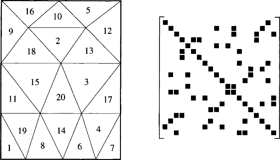
图6.3:二维非结构网格(左)及相应的最近邻模板隐式算子矩阵(右)。图例:左图三角形单元编号1至20;右侧矩阵中非零块矩阵以实心方块表示。
系统矩阵中非零元素的准随机分布是不可取的。它会减慢Gauss-Seidel等迭代求逆方法的收敛速度。此外,ILU(不完全下-上三角分解,Incomplete Lower-Upper)这类Krylov子空间方法的预条件技术也无法高效使用。因此ï¼人们发展了通过对单元(节点)重新编号来大幅减小系统矩阵带宽的策略ï¼即使非零元素聚集到主对角线附近。最著名的重新编号策略是逆Cuthill-McKee(Reverse-Cuthill-McKee,RCM)算法[27]、[28]。图6.4给出了把RCM算法应用于图6.3示例网格后得到的单元编号和系统矩阵。可以看到ï¼矩阵的带宽显著减小ï¼矩阵获得了更规则的结构。en
The quasi-random distribution of nonzero elements in the system matrix is undesirable. It slows down the convergence of iterative inversion methods like Gauss-Seidel. Furthermore, preconditioning techniques for Krylov-subspace methods like ILU (Incomplete Lower-Upper) factorisation scheme cannot be used efficiently. Therefore, strategies were developed where the cells (nodes) are renumbered such that the bandwidth of the system matrix is considerably reduced, i.e., the nonzero elements are clustered close to the main diagonal. The best-known renumbering strategy is the Reverse-Cuthill-McKee (RCM) algorithm [27], [28]. Figure 6.4 shows the resulting cell numbering and the system matrix when the RCM algorithm is applied to the example grid of Fig. 6.3. As we can see, the bandwidth of the matrix is significantly reduced and the matrix obtains a more regular structure.
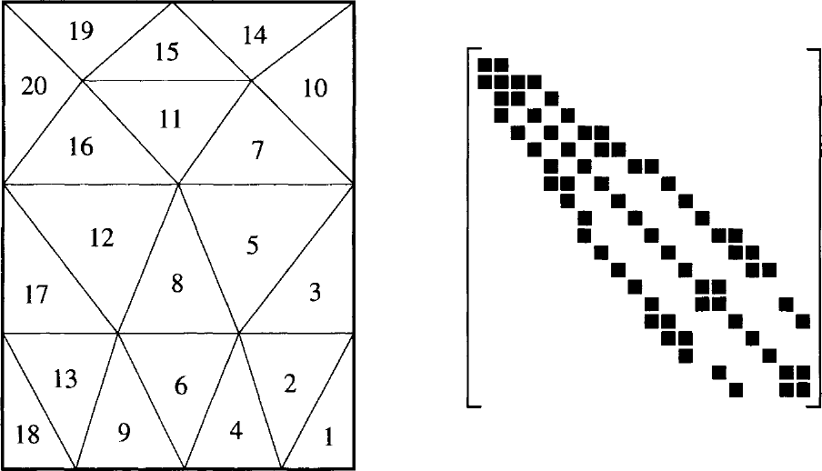
图6.4:用逆Cuthill-McKee(reverse-Cuthill-McKee)排序把图6.3隐式算子的带宽从18减至5。图例:左图为重新编号后的三角形单元网格(编号1至20);右侧矩阵中非零块矩阵以实心方块表示。
为了减少缓存未命中或允许数值格式向量化ï¼还发展了其他一些重新编号策略。综述可参见例如文献[29]。en
Several other renumbering strategies were developed in order to minimise cache misses or to allow for vectorisation of the numerical scheme. An overview can be found, e.g., in Ref. [29].
6.2.2 Evaluation of the Flux Jacobian 通量雅可比的求值[cfd-6-2-2]
视底层空间离散化格式的类型而定ï¼解析求出方程(6.28)中的通量雅可比\(\partial\vec{R}/\partial\vec{W}\)可能非常复杂ï¼甚至不可能。为使概念更清晰ï¼我们先对无黏流动导出通量雅可比ï¼然后再讨论向Navier-Stokes方程的推广。en
Depending on the type of the underlying spatial discretisation scheme, an analytical evaluation of the flux Jacobian \(\partial\vec{R}/\partial\vec{W}\) in Eq. (6.28) may become very complex if not impossible. In order to make the concepts more clear, we shall derive the flux Jacobian for inviscid flows and then discuss the extension to the Navier-Stokes equations.
Central Scheme 中心格式
在中心空间离散化的情形下ï¼通量雅可比最容易构造。如图6.1的例子所示,\(\partial\vec{R}/\partial\vec{W}\)由对流通量雅可比组成(参见方程(6.34))ï¼它们可以解析导出(见A.9节)。人工黏性通常以简化形式纳入ï¼即不含非线性压力传感器(方程(4.55))。这一点将在6.2.3小节再讨论。en
The flux Jacobian is most easily formulated in the case of the central spatial discretisation. As we already saw for the example in Fig. 6.1, \(\partial\vec{R}/\partial\vec{W}\) consists of the convective flux Jacobians (cf. Eq. (6.34)), which can be derived analytically (see Section A.9). Artificial viscosity is usually included in a simplified form, without the non-linear pressure sensor (Eq. (4.55)). We shall return to this point below in Subsection 6.2.3.
Flux-Vector Splitting Scheme 通量向量分裂格式
当以通量向量分裂格式(4.3.2小节)之一为基础来导出通量雅可比时ï¼其求值变得更加复杂。为说明起见ï¼考察Steger和Warming[30]的格式。已有的研究[31]表明ï¼对隐式算子的各种上风离散化,Steger-Warming分裂比例如Van Leer的通量向量分裂格式(方程(4.60))更可取。en
The evaluation of the flux Jacobian becomes more involved when one of the flux-vector splitting schemes (Subsection 4.3.2) is used as the basis for its derivation. Let us, for illustration, consider the scheme due to Steger and Warming [30]. Previous investigations [31] revealed that the Steger-Warming splitting is preferable over, e.g., the Van Leer's flux-vector splitting scheme (Eq. (4.60)) for various upwind discretisations of the implicit operator.
Steger-Warming通量向量分裂格式的基本思想是把对流通量分成正、负两部分ï¼即en
The basic idea of the Steger-Warming flux-vector splitting scheme is to divide the convective fluxes into a positive and a negative part, i.e.,
其中通量定义为en
with the fluxes defined as
在方程(6.37)中,\(\bar{A}_{SW}^{\pm}\)表示正/负Steger-Warming通量分裂雅可比;\(\bar{T}\)表示右特征向量矩阵,\(\bar{T}^{-1}\)为左特征向量矩阵,\(\bar{\Lambda}^{\pm}\)代表正/负特征值构成的对角矩阵(参见A.11节)。特征值矩阵定义为[30]en
In Eq. (6.37), \(\bar{A}_{SW}^{\pm}\) denotes the positive/negative Steger-Warming flux-splitting Jacobian. Furthermore, \(\bar{T}\) represents the matrix of right eigenvectors, \(\bar{T}^{-1}\) the matrix of left eigenvectors, and \(\bar{\Lambda}^{\pm}\) stands for the diagonal matrix of positive/negative eigenvalues, respectively (cf. Section A.11). The eigenvalue matrices are defined as [30]
在上面的方程(6.39)中,\(\Delta\vec{W}_{L,m}^n\)和\(\Delta\vec{W}_{R,m}^n\)分别表示面\(m\)处左状态和右状态的更新量。在结构网格上ï¼左、右状态可以用MUSCL方法(方程(4.46))求值;在非结构网格上ï¼可以采用5.3.3小节讨论的重构方法。然而ï¼模板随精度提高而变宽ï¼导致系统矩阵的带宽增大。因此ï¼也为了降低数值复杂性ï¼方程(6.39)中通常只采用一阶精度近似。作为一种折中ï¼可以用更高精度重构左、右状态ï¼但在求导数时保留一阶格式的模板[32]。en
In the above Eq. (6.39), \(\Delta\vec{W}_{L,m}^n\) and \(\Delta\vec{W}_{R,m}^n\) denote the updates of the left and right state at the face \(m\), respectively. On structured grids, the left and right state can be evaluated by the MUSCL approach (Eq. (4.46)). On unstructured grids, the reconstruction methods discussed in Subsection 5.3.3 can be applied. However, the stencil becomes wider with increasing accuracy, which leads to larger bandwidth of the system matrix. Therefore, and in order to reduce the numerical complexity, only first-order accurate approximation is usually employed in Eq. (6.39). As a compromise, we could reconstruct the left and right state with higher accuracy but retain the stencil of the first-order scheme for the evaluation of the derivatives [32].
对负通量也可以得到与方程(6.40)类似的表达式。可以看到ï¼方程(6.40)的第一项由对流通量雅可比组成(见A.9节)ï¼因而没有困难;但第二项涉及矩阵元素的导数。虽然可以通过手工推导或使用符号代数软件解析地得到这些导数ï¼但这会产生庞大而计算效率低下的代码[33]。另一种可能的做法是假定矩阵\(\bar{A}_c\)局部为常值ï¼从而可以忽略方程(6.40)中的第二项。然而ï¼视隐式格式的类型而定ï¼这可能会严重限制CFL数[34]。en
An expression similar to Eq. (6.40) can also be found for the negative flux. As we can see, the first term in Eq. (6.40) consists of convective flux Jacobians (see Section A.9) and thus presents no difficulty. However, the second term involves derivatives of matrix elements. Although it is possible to obtain the derivatives analytically either by hand calculation or by using a symbolic algebra package, this will produce a large, computationally inefficient code [33]. Alternatively, it is possible to assume the matrix \(\bar{A}_c\) is locally constant so that the second term in Eq. (6.40) can be neglected. However, depending on the type of the implicit scheme, this may severely restrict the CFL number [34].
计算方程(6.39)中导数\(\partial\vec{F}_c^{\pm}/\partial\vec{W}\)的其他可行方法还有源代码的自动微分(例如使用ADIFOR[35])或有限差分法(参见例如[26]、[33])。这样ï¼向量\(\vec{F}\)的第\(i\)个分量对因变量\(\vec{X}\)第\(j\)个分量的导数可以近似为en
Other approaches that we could use to compute the derivatives \(\partial\vec{F}_c^{\pm}/\partial\vec{W}\) in Eq. (6.39) would be the automatic differentiation of the source code (e.g., using ADIFOR [35]) or the finite-difference method (see, e.g., [26], [33]). Herewith, the derivative of the \(i\)-th component of a vector \(\vec{F}\) with respect to the \(j\)-th component of a dependent variable \(\vec{X}\) can be approximated as
其中\(\vec{e}^{\,j}\)表示第\(j\)个标准基向量。Dennis和Schnabel[36]建议步长\(h_j\)取如下形式en
where \(\vec{e}^{\,j}\) denotes the \(j\)-th standard basis vector. Dennis and Schnabel [36] suggested a stepsize \(h_j\) of the form
其中\(\epsilon\)为机器精度,\(\text{typ}\,x_j\)为\(x_j\)的典型大小。关于雅可比矩阵的高效数值求值ï¼还可参阅[37]和[38]中的提示。en
with \(\epsilon\) being the machine accuracy and \(\text{typ}\,x_j\) a typical size of \(x_j\). The reader is also referred to [37] and [38] for hints on efficient numerical evaluation of Jacobian matrices.
Flux-Difference Splitting Scheme 通量差分分裂格式
与通量向量分裂类似ï¼表达式(6.43)既包含对流通量雅可比ï¼也包含Roe矩阵\(\bar{A}_{Roe}\)的导数。这些导数已在[34]中给出。由于相应的公式非常复杂(另见文献[33])ï¼更好的做法是像上文讨论的那样ï¼用数值方法求值\(\partial\vec{F}_c/\partial\vec{W}\)项。en
Similar to flux-vector splitting, the expression (6.43) contains convective flux Jacobians as well as derivatives of the Roe matrix \(\bar{A}_{Roe}\). The derivatives were presented in [34]. Since the corresponding formulae are very complex (see also Ref. [33]), it is a better idea to evaluate the term \(\partial\vec{F}_c/\partial\vec{W}\) numerically, as discussed above.
Viscous Flows 黏性流动
对于Navier-Stokes方程ï¼还必须在隐式算子中计入黏性通量。导数\(\partial\vec{F}_v/\partial\vec{W}\)ï¼即式(6.30)中的黏性通量雅可比ï¼一般不容易直接得到。额外的复杂性来自黏性通量向量本身包含流动变量的导数这一事实。因此ï¼要么用有限差分(式(6.41))求黏性通量雅可比ï¼要么采用简化的形式。en
For the Navier-Stokes equations, we have to account also for the viscous fluxes in the implicit operator. The derivative \(\partial\vec{F}_v/\partial\vec{W}\), i.e., the viscous flux Jacobian in Eq. (6.30) is in general not straightforward to obtain. Additional complexity arises due to the fact that the viscous flux vector contains derivatives of flow variables. For this reason, we have either to evaluate the viscous flux Jacobian by finite differences (Eq. (6.41)), or we have to use a simplified formulation.
在Navier-Stokes方程的TSL近似下(参见2.4.3小节与附录A.6节)ï¼通过假设动力黏度与热传导系数局部为常数ï¼可以解析地求出黏性通量雅可比。于是ï¼根据附录A.10中的讨论ï¼式(6.29)中与黏性通量相关的项变为en
In the case of the TSL approximation of the Navier-Stokes equations (cf. Subsection 2.4.3 and Section A.6), it is possible to find the viscous flux Jacobian analytically by assuming locally constant dynamic viscosity and thermal conductivity coefficients. Then, according to the discussion in Appendix A.10, the term related to the viscous fluxes in Eq. (6.29) becomes
在上式(6.45)中,\(\bar{A}^{*}_v\)表示由式(A.71)或式(A.75)给出的黏性通量雅可比ï¼但不含空间算子\(\partial_y(\cdot)\)(参见式(A.74)与(A.79))。除动力黏度取算术平均外ï¼这些雅可比对其余所有变量要么用左状态、要么用右状态求值。应当指出ï¼假如左右状态以一阶精度计算ï¼式(6.45)在隐式算子中给出的是二阶中心差分近似。en
In above Eq. (6.45), \(\bar{A}^{*}_v\) stands for the viscous flux Jacobian given by Eq. (A.71) or Eq. (A.75) but without the spatial operators \(\partial_y(\cdot)\) (cf. Eq. (A.74) and (A.79)). The Jacobians are evaluated using either the left or the right state for all variables except for the dynamic viscosity, which is determined from an arithmetic average. It should be mentioned that Eq. (6.45) leads to a second-order central difference approximation in the implicit operator, supposed the left and right state are computed with first-order accuracy.
6.2.3 ADI Scheme ADI格式[cfd-6-2-3]
交替方向隐式(Alternating Direction Implicit,ADI)格式是最早的迭代式隐式格式之一[40]。ADI格式只能在结构网格上实现。它基于把式(6.28)中的隐式算子近似分裂(或者说ï¼因式分解)为二维时的两个、三维时的三个因子。每个因子包含计算空间中某一特定方向的对流通量与黏性通量的线性化。在三维情形ï¼这导出如下形式[40]、[41]en
The Alternating Direction Implicit (ADI) scheme was one of the first iterative implicit schemes [40]. The ADI scheme can be implemented on structured grids only. It is based on an approximate splitting (or, in other words, factorisation) of the implicit operator in Eq. (6.28) into two (in 2D) or three (in 3D) factors. Each factor contains the linearisation of the convective and viscous fluxes for one particular direction in the computational space. In 3D, this leads to the formulation [40], [41]
为清晰起见ï¼式(6.46)中在不必要之处省略了节点指标\(i\)、\(j\)、\(k\)。此外ï¼式(6.46)中的上标\(I\)、\(J\)、\(K\)标记与计算空间中某一坐标相关联的通量向量或面面积。例如,\(\Delta S^{I}_{i+1/2,j,k}\)对应于图4.1b中的\(\Delta S_2\)。把节点指标换成单元指标ï¼式(6.46)的格式即可用于单元中心离散。en
For clarity, the node indices \(i, j, k\) were omitted from Eq. (6.46) where not required. Furthermore, the superscripts \(I, J, K\) in Eq. (6.46) mark the flux vector or of the face area associated with certain coordinate in the computational space. For example, \(\Delta S^{I}_{i+1/2,j,k}\) corresponds to \(\Delta S_2\) in Fig. 4.1b. By replacing the node indices by cell indices, the scheme in Eq. (6.46) can be applied to a cell-centred discretisation.
式(6.46)中对流通量与黏性通量的导数可以按上一小节所讨论的方法计算。ADI方法传统上与带人工耗散的中心格式耦合使用。在这种情形下ï¼每个因子都具有与式(6.34)类似的形式(当然ï¼源项的线性化只包含在一个因子中)。为了得到稳健而高效的格式ï¼必须在隐式算子中纳入人工耗散项的线性化[42]-[44]。该线性化一般通过把谱半径与耗散系数视为与\(\vec{W}\)无关来简化。于是ï¼根据式(4.48)ï¼例如I方向上的因子变为en
The derivatives of the convective and viscous fluxes in Eq. (6.46) can be evaluated as discussed in the previous subsection. The ADI method is traditionally coupled to the central scheme with artificial dissipation. In such a case, a formulation similar to that in Eq. (6.34) holds for each factor (of course, the linearisation of the source term is included in one factor only). In order to obtain a robust and efficient scheme, it is necessary to include a linearisation of the artificial dissipation terms in the implicit operator [42]-[44]. The linearisation is in general simplified by treating the spectral radii and the dissipation coefficients as independent of \(\vec{W}\). Hence, according to Eq. (4.48) the factor, e.g., in the I-direction becomes
其中的隐式人工耗散项按JST格式(参见式(4.50))为en
with the implicit artificial dissipation term JST scheme, (cf. Eq. (4.50))
其他方向的隐式耗散项按类似方式定义。也可以在隐式算子中只保留二阶差分[43]、[44]。这会把每个因子的矩阵从块五对角形式约化为块三对角形式(如图6.1所示意)。然而ï¼正如文献[44]所指出的ï¼这会限制格式的稳定性。en
The implicit dissipation terms in other directions are defined in similar way. It is also possible to retain only the second-order differences in the implicit operator [43], [44]. This reduces the matrix for each of the factors from block-pentadiagonal to block-tridiagonal form (as sketched in Fig. 6.1). However, as pointed out in Ref. [44], this restricts the stability of the scheme.
其中\(\mathbf{D}\)表示对角项,\(\mathbf{L}\)表示下对角项,\(\mathbf{U}\)表示上对角项。每一步都需要对块三对角或块五对角矩阵求逆(若式(6.47)中的\(\epsilon^{(4)}_{IM} > 0\))。这由直接解法完成。为了减少数值工作量,Pulliam与Chaussee[45]提出了ADI格式的对角化形式。由此ï¼块矩阵(由对流通量与黏性通量雅可比组成)被变换为对角矩阵。于是只需对非块的三对角或五对角矩阵求逆ï¼可显著节省计算量与内存[43]。虽然这种对角化严格来说只对欧拉方程成立ï¼但它同样可用于黏性流动[43]。此时ï¼黏性通量的线性化(例如式(6.45)那样)要么在隐式算子中省略ï¼要么可以用黏性特征值(式(6.19))来近似。en
where \(\mathbf{D}\) represents the diagonal, \(\mathbf{L}\) the lower-diagonal and \(\mathbf{U}\) the upper-diagonal terms, respectively. Each step requires the inversion of a block-tridiagonal or a block-pentadiagonal matrix (if \(\epsilon^{(4)}_{IM} > 0\) in Eq. (6.47)). This is done by a direct solution method. In order to reduce the numerical effort, Pulliam and Chaussee [45] suggested a diagonalised form of the ADI scheme. Herewith, the block matrices (composed of convective and viscous flux Jacobians) are transformed into diagonal matrices. Hence, only non-block tri- or pentadiagonal matrices have to be inverted, which results in significant savings of computational work and memory [43]. Although the diagonalisation is strictly valid only for Euler equations, it can be employed for viscous flows as well [43]. The linearisation of the viscous fluxes (e.g., like in Eq. (6.45)) is then either omitted in the implicit operator, or it can be approximated by the viscous eigenvalue (Eq. (6.19)).
对隐式算子的分裂引入了所谓的因式分解误差(factorisation error)。它是式(6.28)基本格式的隐式算子与因式分解后算子之差。对ADI格式而言ï¼该误差项以因子\((\Delta t)^{N}\)缩放ï¼其中\(N\)为空间维数。这一项使ADI格式在三维中失去无条件稳定性[46]。不过ï¼如果把人工黏性的四阶差分包含在隐式算子中ï¼稳定性会得到改善[44]。事实上,ADI格式已被成功地用于求解各种三维问题[43]、[47]。Rosenfeld等人[48]提出了一种在多块网格上隐式处理块边界的ADI格式的有趣实现。en
The splitting of the implicit operator introduces what is called the factorisation error. It is the difference between the implicit operator of the base scheme in Eq. (6.28) and the factorised operator. In the case of the ADI scheme, this error term is scaled by the factor \((\Delta t)^{N}\), where \(N\) denotes the number of space dimensions. This term causes the ADI scheme to loose its unconditional stability in 3D [46]. However, the stability is improved if the fourth-order differences of the artificial viscosity are included in the implicit operator [44]. In fact, the ADI scheme was successfully used for the solution of various 3-D problems [43], [47]. An interesting implementation of the ADI scheme on multiblock grids, which treats the block boundaries implicitly, was presented by Rosenfeld et al. [48].
6.2.4 LU-SGS Scheme LU-SGS格式[cfd-6-2-4]
隐式下-上对称Gauss-Seidel(Lower-Upper Symmetric Gauss-Seidel,LU-SGS)格式ï¼也称为下-上对称逐次超松弛(Lower-Upper Symmetric Successive Overrelaxation,LU-SSOR)格式ï¼因其数值复杂度低、内存需求适中——两者均与显式多级格式相当——而得到广泛使用。此外,LU-SGS格式易于在向量机与并行计算机上实现ï¼既可用于结构网格ï¼也可用于非结构网格。en
The implicit Lower-Upper Symmetric Gauss-Seidel (LU-SGS) scheme, which is also called the Lower-Upper Symmetric Successive Overrelaxation (LU-SSOR) scheme, became widely-used because of its low numerical complexity and modest memory requirements, which are both comparable to an explicit multistage scheme. Furthermore, the LU-SGS scheme can be implemented easily on vector and parallel computers. It can also be used on structured as well as on unstructured grids.
LU-SGS格式源于Jameson与Turkel[49]的工作ï¼他们研究了把隐式算子分解为下、上对角占优因子的方法。LU-SGS方法本身由Yoon与Jameson[50]-[52]提出ï¼作为求解式(6.28)未分解隐式格式的一种松弛方法。Rieger与Jameson[53]进一步发展了该方法并将其应用于三维黏性流场。此后ï¼多位研究者把LU-SGS格式应用于结构网格[54]-[61]与非结构网格[62]-[66]上的黏性流动。LU-SGS方法也常用于化学反应流动的模拟[67]-[71]。en
The LU-SGS scheme has its origins in the work of Jameson and Turkel [49], who considered decompositions of the implicit operator into lower and upper diagonally dominant factors. The LU-SGS method itself was introduced by Yoon and Jameson [50]-[52] as a relaxation method for solving the unfactored implicit scheme in Eq. (6.28). It was further developed and applied to 3-D viscous flow fields by Rieger and Jameson [53]. Since then, various researchers applied the LU-SGS scheme to viscous flows on structured [54]-[61] and on unstructured grids [62]-[66]. The LU-SGS approach is often used for the simulation of chemically reacting flows [67]-[71].
对于式(6.29)中对流通量的线性化,LU-SGS格式采用Steger与Warming(见6.2.2小节)一阶精度通量向量分裂方法的一种简化形式。无论显式算子如何离散ï¼该线性化始终保持不变。此外,LU-SGS格式基于把式(6.28)的隐式算子因式分解为以下三部分en
The LU-SGS scheme employs a simplification of the first-order accurate flux-vector splitting approach due to Steger and Warming (see Subsection 6.2.2) for the linearisation of the convective fluxes in Eq. (6.29). The linearisation is always kept the same regardless of the discretisation of the explicit operator. The LU-SGS scheme is further based on the factorisation of the implicit operator in Eq. (6.28) into the following three parts
这些因子的构造使得\(\mathbf{L}\)只包含严格下三角矩阵中的项,\(\mathbf{U}\)只包含严格上三角矩阵中的项ï¼而\(\mathbf{D}\)只包含对角项。值得注意的是ï¼因子的数目始终保持不变ï¼与空间维数无关。en
The factors are constructed such that \(\mathbf{L}\) consists only of terms in the strictly lower triangular matrix, \(\mathbf{U}\) of terms in the strictly upper triangular matrix and \(\mathbf{D}\) of diagonal terms. It is important to remark that the number of factors remains always the same independent of the number of space dimensions.
其中\(\vec{W}^{n+1} = \vec{W}^{n} + \Delta\vec{W}^{n}\)。算子\(\mathbf{L}\)、\(\mathbf{D}\)、\(\mathbf{U}\)以及求逆过程在结构网格与非结构网格上存在若干差异。因此ï¼下面分别讨论这两种情形。en
with \(\vec{W}^{n+1} = \vec{W}^{n} + \Delta\vec{W}^{n}\). The operators \(\mathbf{L}\), \(\mathbf{D}\), and \(\mathbf{U}\) and also the inversion procedure differ on structured and unstructured grids in some respects. Therefore, we shall discuss below each case separately.
LU-SGS on Structured Grids 结构网格上的LU-SGS
在结构网格上ï¼算子定义为(参见[50]-[52]以及[68]、[55])en
On structured grids, the operators are defined as (see [50]-[52], and [68], [55])
为了便于阅读ï¼式(6.51)中只标出了与\(i\)、\(j\)、\(k\)不同的那些节点指标(单元中心格式下为单元指标)。\(\Delta S\)上的上标\(i\)、\(j\)、\(k\)指示计算空间中的方向。正/负通量雅可比\(\bar{A}^{\pm}\)以及黏性通量雅可比\(\bar{A}_{v}\)中的单位法向量ï¼与相关联的面面积\(\Delta S\)一样ï¼在控制体的同一侧取值。注意ï¼这里假定单位法向量指向控制体外侧。相反ï¼在各种文献中则假定控制体相对两侧的单位法向量指向同一方向。en
For better readability, only those node indices (or cell indices in the case of a cell-centred scheme) are shown in Eq. (6.51), which differ from \(i, j, k\). The superscripts \(i, j, k\) at \(\Delta S\) indicate the direction in the computational space. The unit normal vectors in the positive/negative flux Jacobians \(\bar{A}^{\pm}\) and in the viscous flux Jacobians \(\bar{A}_{v}\) are evaluated at the same side of the control volume like the associated face areas \(\Delta S\). Note that the unit normal vectors are assumed to point outwards of the control volume. In contrast, in various references it is supposed that the unit normal vectors from opposite sides of the control volume point in the same direction.
式(6.51)中的黏性通量雅可比要么数值计算ï¼要么按式(6.45)用其TSL近似代替。无论边界层的实际取向如何ï¼都可以在所有计算坐标上应用TSL近似。进一步的简化是把黏性通量雅可比用黏性谱半径(式(6.19))代替ï¼即\(\bar{A}_{v}\Delta S \approx \hat{\Lambda}_{v}\)ï¼如文献[63]所建议。en
The viscous flux Jacobians in Eq. (6.51) are either computed numerically, or are replaced by their TSL approximation, corresponding to Eq. (6.45). It is possible to apply the TSL approximation in all computational coordinates, regardless of the actual orientation of the boundary layer(s). A further simplification consists of substituting the viscous flux Jacobians by the viscous spectral radii (Eq. (6.19)), i.e., \(\bar{A}_{v}\Delta S \approx \hat{\Lambda}_{v}\), as suggested in [63].
分裂的对流通量雅可比\(\bar{A}^{\pm}\)的构造方式是:(+)矩阵的特征值全部非负,(-)矩阵的特征值全部非正。一般地ï¼这些矩阵定义为[49]en
The split convective flux Jacobians \(\bar{A}^{\pm}\) are constructed in such a way that the eigenvalues of the (+) matrices are all non-negative, and of the (-) matrices are all non-positive. In general, the matrices are defined as [49]
其中\(\bar{A}_{c}\)为对流通量雅可比(见A.9节),\(\hat{\Lambda}_{c}\)为对流通量雅可比的谱半径(由式(4.53)或式(6.15)给出)。当忽略\(\bar{A}_{c}\)的导数时ï¼上述近似(6.52)与式(6.40)相似。式(6.52)中的因子\(\omega\)为超松弛参数ï¼它同时决定隐式耗散的量ï¼从而影响格式的收敛特性。该因子可在\(1 < \omega \le 2\)范围内选取。\(\omega\)值越高,LU-SGS格式的稳定性越好ï¼但可能减慢到定态的收敛。式(6.52)中雅可比\(\bar{A}^{\pm}\)的定义保证了系统矩阵对角占优ï¼这对迭代求逆过程(6.50)的效率与稳健性非常重要。en
where \(\bar{A}_{c}\) stands for the convective flux Jacobian (Section A.9) and \(\hat{\Lambda}_{c}\) represents the spectral radius of the convective flux Jacobian (given by Eq. (4.53) or Eq. (6.15)), respectively. Note the similarity between the above approximation (6.52) and Eq. (6.40), when the derivatives of \(\bar{A}_{c}\) are neglected. The factor \(\omega\) in Eq. (6.52) represents an overrelaxation parameter. It also determines the amount of implicit dissipation and hence influences the convergence properties of the scheme. The factor can be chosen in the range \(1 < \omega \le 2\). Higher values of \(\omega\) increase the stability of the LU-SGS scheme, but may slow down the convergence to steady state. The definition of the Jacobians \(\bar{A}^{\pm}\) in Eq. (6.52) ensures a diagonally dominant system matrix, which is very important for the efficiency and robustness of the iterative inversion procedure (6.50).
对流通量雅可比的谱半径\(\hat{\Lambda}_{c}\)由式(6.15)给出。面面积与法向量分别按式(6.16)在I、J或K方向上作平均。正如马上将看到的ï¼这一近似有助于显著减少运算量与内存需求。en
The spectral radii of the convective flux Jacobians \(\hat{\Lambda}_{c}\) are given in Eq. (6.15). The face areas and normal vectors are averaged in the respective I-, J-, or K-direction according to Eq. (6.16). As we shall see immediately, this approximation helps to reduce the operation count and the memory requirements significantly.
LU-SGS方法的一个显著特点在于式(6.50)中前扫与后扫的执行方式。在二维中ï¼扫掠沿计算空间中的对角线\((i+j) = \mathrm{const.}\)进行。图6.5描绘了前扫(式(6.50)第一行)的情形。这样,\(\mathbf{L}\)算子与\(\mathbf{U}\)算子所涉及的非对角项便可以从扫掠的前一部分获得(在图6.5中用叉号表示)。在三维中ï¼隐式算子在\(i+j+k = \mathrm{const.}\)平面上求逆ï¼如图6.6所示意。于是,LU-SGS格式可以写为en
A distinguishing feature of the LU-SGS method is how the forward and the backward sweep in Eq. (6.50) are carried out. In 2D, the sweeps are accomplished along diagonal lines \((i+j) = \mathrm{const.}\) in computational space. This is depicted in Fig. 6.5 for the forward sweep (first line of Eq. (6.50))). In this way, the off-diagonal terms involved in the \(\mathbf{L}\) and the \(\mathbf{U}\) operator become known from the previous part of a sweep (denoted by crosses in Fig. 6.5). In 3D, the implicit operator is inverted on \(i+j+k = \mathrm{const.}\) planes, as sketched in Fig. 6.6. Hence, the LU-SGS scheme can be written as
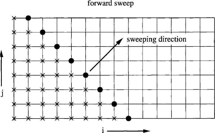
图6.5:LU-SGS格式在计算空间中的扫掠方向。图例:\(\bullet\)表示算子\(\mathbf{D}\)当前被求逆的位置(直线\(i+j=\mathrm{const.}\));\(\times\)表示\(\mathbf{L}\)的已更新值。
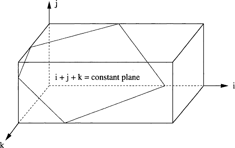
图6.6:三维隐式LU-SGS格式扫掠的对角面。图内标注:\(i+j+k\)=常数平面(i+j+k = constant plane)。
由式(6.54)可见ï¼唯一需要求逆的是对角项\(\mathbf{D}\)。这样,LU-SGS方法把稀疏带状矩阵的求逆转化为块对角矩阵的求逆。此外ï¼若式(6.53)中的黏性通量雅可比用黏性谱半径近似ï¼算子\(\mathbf{D}\)便成为对角矩阵(源项除外)。因此ï¼与其他隐式格式(例如前面讨论过的ADI格式)相比,LU-SGS格式所需的计算量非常小。而且ï¼对角算子的求逆可以对角面上的每个节点(单元)独立进行ï¼这使该格式易于向量化。对角面上节点/单元的指标可用如下伪代码获得[72]:en
As we can see from Eq. (6.54), the only term which needs to be inverted is the diagonal term \(\mathbf{D}\). Thus, the LU-SGS methodology transforms the inversion of a sparse banded matrix into the inversion of a block-diagonal matrix. Furthermore, if the viscous flux Jacobians in Eq. (6.53) are approximated by the viscous spectral radii, the operator \(\mathbf{D}\) becomes a diagonal matrix (except for the source term). Hence, the LU-SGS scheme requires a very small computational effort as compared to other implicit schemes (e.g., the ADI scheme discussed previously). Furthermore, the inversion of the diagonal operator can be carried out independently for each node (cell) of the diagonal plane, which makes the scheme easy to vectorise. The indices of the nodes/cells on the diagonal planes can be obtained with the following pseudo-code [72]:
    DO plane = 1, nplanes
       DO k = 1, kmax
          DO j = 1, jmax
             DO i = 1, imax
                IF (i+j+k = plane+2) store indices
             ENDDO
          ENDDO
       ENDDO
    ENDDO
对角面的数目为:nplanes = imax + jmax + kmax - 2。显然ï¼为了获得更高的计算效率ï¼可对上述代码进行优化。en
nplanes = imax + jmax + kmax - 2。显然ï¼为了获得更高的计算效率ï¼可对上述代码进行优化。enThe number of diagonal planes is: nplanes = imax + jmax + kmax - 2. Obviously, the above code can be optimised for higher computational efficiency.
为了避免在\(\mathbf{L}\)与\(\mathbf{U}\)中显式计算并存储对流通量雅可比ï¼乘积\(\bar{A}^{\pm}\Delta\vec{W}^{n}\)可以用通量的Taylor级数展开代替[53]。利用式(6.52)ï¼可以写出en
In order to avoid explicit evaluation and storage of the convective flux Jacobians in \(\mathbf{L}\) and \(\mathbf{U}\), the products \(\bar{A}^{\pm}\Delta\vec{W}^{n}\) can be substituted by Taylor series expansion of the fluxes [53]. Using Eq. (6.52), we can write
其中对流通量的更新为en
with the update of the convective fluxes
由于是沿对角面扫掠,\(\vec{F}^{n+1}_{c}\)此时已知ï¼式(6.55)给出的简化才成为可能。这使LU-SGS格式的数值工作量进一步显著下降。en
The simplification given by Eq. (6.55) is possible due to the sweeping along diagonal planes, since \(\vec{F}^{n+1}_{c}\) is then known. This leads to a further significant decrease of the numerical effort of the LU-SGS scheme.
时间步长\(\Delta t\)可以按6.1.4小节所述方法、用式(6.14)计算。但应注意ï¼如Rieger与Jameson[53]所述ï¼当\(\Delta t \to \infty\)时ï¼式(6.49)的隐式LU-SGS格式代表一次近似Newton迭代。因此ï¼实践中对定常流动一般使用\(10^{4}\)到\(10^{6}\)量级的CFL数。此时收敛由超松弛参数\(\omega\)控制。对于非定常流动的模拟ï¼可以采用下文6.3节给出的形式;另一种可能是使用文献[73]所述的LU-SGS格式的修正版本。en
The time step \(\Delta t\) can be computed in the same way as presented in Subsection 6.1.4, using Eq. (6.14). However, it should be noted that the implicit LU-SGS scheme in Eq. (6.49) represents an approximate Newton iteration in the case of \(\Delta t \to \infty\) as stated by Rieger and Jameson [53]. Thus in general, CFL numbers of the order of \(10^{4}\) to \(10^{6}\) are used in practice for stationary flows. The convergence is then controlled by the overrelaxation parameter \(\omega\). For the simulation of unsteady flows, we may employ the formulation presented below in Section 6.3. Another possibility is to use the modified version of the LU-SGS scheme described in Ref. [73].
LU-SGS on Unstructured Grids 非结构网格上的LU-SGS
这里ï¼对中位对偶(median-dual)格式ï¼算子为[63]-[65]en
Here, the operators read for a median-dual scheme [63]-[65]
在式(6.57)中,\(L(i)\)与\(U(i)\)表示属于下(上)矩阵的节点\(i\)的最近邻节点,\(\Delta S_{ij}\)表示与边\(ij\)相关联的面面积(见图5.9),\(N_{F}\)表示控制体\(\Omega_{i}\)的面数。对流通量的谱半径\((\hat{\Lambda}_{c})_{i}\)由式(6.21)计算。黏性通量雅可比\(\bar{A}_{v}\)同样可以用其谱半径近似[63]。此时ï¼对角算子变为en
In Eq. (6.57), \(L(i)\), and \(U(i)\) denote the nearest neighbours of node \(i\) which belong to the lower (upper) matrix, \(\Delta S_{ij}\) represents the face area associated with the edge \(ij\) (see Fig. 5.9), and \(N_{F}\) stands for the number of faces of the control volume \(\Omega_{i}\), respectively. The spectral radius of the convective fluxes \((\hat{\Lambda}_{c})_{i}\) is computed by Eq. (6.21). The viscous flux Jacobian \(\bar{A}_{v}\) can be again approximated by its spectral radius [63]. In this case, the diagonal operator becomes
其中\((\hat{\Lambda}_{v})_{i}\)按式(6.21)计算。对单元中心格式ï¼可以得到与式(6.57)、(6.58)类似的公式ï¼主要区别是\(\mathbf{L}\)与\(\mathbf{U}\)算子中的求和遍及单元的各个面而非相邻边。en
where \((\hat{\Lambda}_{v})_{i}\) is evaluated according to Eq. (6.21). Formulae similar to Eq. (6.57) and (6.58) can be obtained in the case of the cell-centred scheme. The major difference is that the summation in the \(\mathbf{L}\) and the \(\mathbf{U}\) operator is conducted over faces of the cell instead of incident edges.
式(6.57)中的集合\(L(i)\)与\(U(i)\)应起到与结构网格上对角面相同的作用。为此ï¼必须把节点(单元)划分为层ï¼使得[63]:
- 当前层的节点\(i\)(单元\(I\))与流动变量已更新的层相连——否则LU-SGS格式退化为Jacobi迭代;
- 同一层内的节点(单元)彼此不相连——否则该格式无法向量化。
en
The sets \(L(i)\) and \(U(i)\) in Eq. (6.57) should fulfil the same function as the diagonal planes on structured grids. For this reason, it is necessary to arrange the nodes (cells) into layers such that [63]:
- nodes \(i\) (cells \(I\)) of a current layer have connections to layers with previously updated flow variables - otherwise the LU-SGS scheme degenerates to a Jacobi iteration,
- nodes (cells) in a layer are not connected to each other - otherwise the scheme could not be vectorised.
对中位对偶格式ï¼可按文献[63]所述的方法生成分层;单元中心格式的做法见于[74]、[75]。en
The layers can be generated for the median-dual scheme with a procedure described in Ref. [63]. Approaches for the cell-centred scheme were suggested in [74], [75].
恰当定义集合\(L(i)\)与\(U(i)\)后ï¼可实现如下两步求逆过程[63]-[65]en
An appropriate definition of the sets \(L(i)\) and \(U(i)\) allows for the following two-step inversion procedure [63]-[65]
其中\(\|\vec{r}_{j} - \vec{r}_{i}\|_{2}\)为边\(ij\)的长度。en
with \(\|\vec{r}_{j} - \vec{r}_{i}\|_{2}\) being the length of the edge \(ij\).
时间步长可按显式格式(式(6.20)))同样方式计算。但应略去黏性特征值ï¼因为黏性项已包含在隐式算子中ï¼不会像显式格式那样减小时间步长。对定常流动,CFL数可在\(10^{4}\)到\(10^{6}\)范围内选取。随后可用超松弛参数\(\omega\)来调节LU-SGS格式的收敛速度与稳健性。en
The time step can be computed in the same way as for the explicit scheme (Eq. (6.20))). However, the viscous eigenvalue should be omitted, since the viscous terms are already contained in the implicit operator and hence do not reduce the time step as in the case of an explicit scheme. The CFL number can be chosen in the range from \(10^{4}\) to \(10^{6}\) for steady flows. The convergence speed and the robustness of the LU-SGS scheme can then be tuned using the overrelaxation parameter \(\omega\).
6.2.5 Newton-Krylov Method Newton-Krylov方法[cfd-6-2-5]
其中\(\bar{J}\)表示隐式算子(系统矩阵)。如前所述,\(\bar{J}\)是一个大型、稀疏且一般非对称的矩阵。在前几小节中ï¼我们讨论了把\(\bar{J}\)分解为若干因子的两种方法ï¼每个因子都比\(\bar{J}\)本身更易求逆。然而ï¼由于因式分解误差(以及\(\vec{R}^{n+1}\)的近似线性化)ï¼只能获得到定态的线性收敛。为了得到求解非线性方程的Newton法的二次收敛ï¼必须满足四个条件:
- 残差的线性化必须精确;
- \(\bar{J}\)必须被准确求逆;
- 时间步长须为\(\Delta t \to \infty\);
- 初始解在某种意义上必须接近最终解。
en
where \(\bar{J}\) represents the implicit operator (system matrix). As we already saw, \(\bar{J}\) constitutes a large, sparse, and generally non-symmetric matrix. In the previous subsections, we discussed two methods that decompose \(\bar{J}\) into several factors which can be each more easily inverted than \(\bar{J}\) itself. However, due to the factorisation error (and approximate linearisation of \(\vec{R}^{n+1}\)), only a linear convergence to steady state can be achieved. In order to obtain the quadratic convergence of Newton's method for the solution of non-linear equations, four conditions must be fulfilled:
- the linearisation of the residual must be exact,
- \(\bar{J}\) must be accurately inverted,
- the time step has to be \(\Delta t \to \infty\),
- initial solution must be, in some sense, close to the final solution.
显然ï¼必须克服的主要障碍是完整系统矩阵的线性化与求逆。en
Obviously, the main obstacles that have to be overcome are the linearisation and the inversion of the full system matrix.
对求解大型线性方程组而言ï¼一类特别合适的迭代技术是所谓的Krylov子空间(Krylov-subspace)方法。针对CFD中出现的矩阵求逆ï¼已有若干方法被提出ï¼例如平方共轭梯度(Conjugate Gradient Squared,CGS)法[76]、稳定双共轭梯度(Bi-Conjugate Gradient Stabilised,Bi-CGSTAB)格式[77]ï¼以及无转置准最小残差(Transpose-Free Quasi-Minimum Residual,TFQMR)方法[78]。然而ï¼最成功的Krylov子空间方法是广义最小残差(Generalised Minimal Residual,GMRES)技术ï¼它最初由Saad与Schulz[79]、[80]提出。此后,GMRES方法被多位研究者改进与扩充[81]-[84]。由于其流行程度ï¼下面将重点讨论GMRES方法。尽管如此ï¼我们将讨论的大部分内容同样适用于其他Krylov子空间方法。en
A particularly suitable class of iterative techniques for the solution of large linear equation systems are the so-called Krylov-subspace methods. Several were proposed for the inversion of matrices which arise in CFD. Examples are the Conjugate Gradient Squared (CGS) method [76], the Bi-Conjugate Gradient Stabilised (Bi-CGSTAB) scheme [77], or the Transpose-Free Quasi-Minimum Residual (TFQMR) approach [78]. However, the most successful Krylov subspace method became the Generalised Minimal Residual (GMRES) technique, which was originally suggested by Saad and Schulz [79], [80]. Since then, the GMRES method was improved and augmented by several researchers [81]-[84]. Because of its popularity, we shall focus on the GMRES approach in the following. Nevertheless, most of what we shall discuss also applies to the other Krylov subspace methods.
GMRES Method GMRES方法
如3.2.2小节所述(另见附录A.12),GMRES方法在一组\(m\)个正交归一向量(搜索方向)上最小化全局残差的范数ï¼即\(\|\bar{J}\Delta\vec{W}^{n} + \vec{R}^{n}\|\)ï¼这些向量张成式(3.10)给出的Krylov子空间\(\mathcal{K}_{m}\)。GMRES算法可概括如下:
- 猜测起始解\(\Delta\vec{W}^{n}_{0}\)并计算初始残差向量\(\vec{r}_{0} = \bar{J}\Delta\vec{W}^{n}_{0} + \vec{R}^{n}\);
- 生成\(m\)个搜索方向(通过Gram-Schmidt正交化);
- 求解最小化问题;
- 构造式(6.61)的近似解\(\Delta\vec{W}^{n} = \Delta\vec{W}^{n}_{0} + \vec{y}_{m}\)。
en
As we mentioned in Subsection 3.2.2 (see also Appendix A.12), the GMRES method minimises the norm of the global residual, i.e., \(\|\bar{J}\Delta\vec{W}^{n} + \vec{R}^{n}\|\) over a set of \(m\) orthonormal vectors (search directions), which span the Krylov subspace \(\mathcal{K}_{m}\) given by Eq. (3.10). The GMRES algorithm can be summarised as follows:
- guess a starting solution \(\Delta\vec{W}^{n}_{0}\) and evaluate the initial residual vector \(\vec{r}_{0} = \bar{J}\Delta\vec{W}^{n}_{0} + \vec{R}^{n}\),
- generate the \(m\) search directions (by Gram-Schmidt orthogonalisation),
- solve the minimisation problem,
- form an approximate solution of Eq. (6.61) as \(\Delta\vec{W}^{n} = \Delta\vec{W}^{n}_{0} + \vec{y}_{m}\).
由于内存需求随搜索方向数目线性增长ï¼实践中\(m\)被限制在10到40之间。这对收敛解\(\Delta\vec{W}^{n}\)而言可能并不足够。因此,GMRES方法必须重启ï¼即令\(\Delta\vec{W}^{n}_{0} = \Delta\vec{W}^{n}\)ï¼计算\(\vec{r}_{0}\)ï¼然后从第2步继续。文献[85]指出ï¼与其使用固定数目的搜索方向ï¼不如在全局残差范数降到给定容差以下时减小\(m\)。这样可以在Newton迭代的后期阶段节省大量运算。en
Since the memory requirements increase linearly with the number of search directions, \(m\) is restricted to values between 10 and 40 in practice. This might not be sufficient for a converged solution \(\Delta\vec{W}^{n}\). Thus, the GMRES method has to be restarted, i.e., we set \(\Delta\vec{W}^{n}_{0} = \Delta\vec{W}^{n}\), compute \(\vec{r}_{0}\) and proceed with step 2. As pointed out in Ref. [85], instead of working with a constant number of search directions, \(m\) should be reduced if the norm of the global residual drops below a specified tolerance. In this way, a large number of operations can be saved in later stages of the Newton iteration.
Computation of the Flux Jacobian 通量雅可比的计算
GMRES及其他Krylov子空间方法使我们得以避免显式计算与存储通量雅可比\(\partial\vec{R}/\partial\vec{W}\)。其想法基于如下观察:这些方法只依赖形如\(\bar{J}\Delta\vec{W}^{n}\)的矩阵-向量乘积ï¼并不需要矩阵\(\bar{J}\)本身。通量雅可比与解更新的乘积可以用简单的有限差分近似为en
GMRES and other Krylov subspace methods allow us to circumvent an explicit computation and storage of the flux Jacobian \(\partial\vec{R}/\partial\vec{W}\). The idea is based on the observation that the methods rely only on matrix-vector products of the form \(\bar{J}\Delta\vec{W}^{n}\) and do not need the matrix \(\bar{J}\) explicitly. The product of the flux Jacobian with the solution update can be approximated by a simple finite difference as
这只需要两次残差计算。为了使数值误差最小ï¼步长\(h\)的选择需要相当谨慎[36]。一种特别合适的公式为[86]en
which requires only two evaluations of the residual. The stepsize \(h\) has to be chosen with some care, in order to minimise the numerical error [36]. One particularly suitable formulation reads [86]
其中\(\epsilon\)为机器精度,\(d\)为标量积\(\vec{W}^{n}\cdot\Delta\vec{W}^{n}\),\(|\Delta\vec{W}^{n}|\)是所有元素取绝对值后的向量\(\Delta\vec{W}^{n}\)ï¼而\(\mathrm{typ}\,U\)表示\(U\)的典型大小。除了节省内存与运算量之外ï¼有限差分近似还有一个更重要的优点:可以容易地实现对高阶残差\(\vec{R}^{n}\)(包括边界条件、限制器、源项等)在数值上精确的线性化。en
where \(\epsilon\) denotes the machine accuracy, \(d\) the scalar product \(\vec{W}^{n}\cdot\Delta\vec{W}^{n}\), \(|\Delta\vec{W}^{n}|\) is the vector \(\Delta\vec{W}^{n}\) with all elements set to their absolute values, and finally \(\mathrm{typ}\,U\) represents a typical size of \(U\). Apart from saving memory and operations, there is an even more important advantage of the finite-difference approximation. Namely, numerically accurate linearisation of a high-order residual \(\vec{R}^{n}\) (including boundary conditions, limiters, source terms, etc.) can be easily achieved.
这样,Newton格式的二次收敛便能以适度的代价实现。因此ï¼我们把这类格式称为Newton-Krylov方法[86]-[88]。en
Thus, the quadratic convergence of Newton's scheme can be realised at moderate costs. For this reason, we speak of such a scheme as of Newton-Krylov approach [86]-[88].
Preconditioning 预条件
Krylov子空间方法的效率在很大程度上依赖于一个好的预条件子。其目的是使系统矩阵\(\bar{J}\)的特征值聚集在1附近。于是ï¼不再求解方程(6.61)ï¼而是按式(3.11)求解左预条件或右预条件系统。把式(6.61)与式(6.62)同条件\(\Delta t \to \infty\)相结合,Newton-Krylov方法成为en
The efficiency of Krylov-subspace methods depends strongly on a good preconditioner. Its purpose is to cluster the eigenvalues of the system matrix \(\bar{J}\) around unity. Thus, instead of Equation (6.61), the left- or right-preconditioned system according to Eq. (3.11) is solved. Using Eqs. (6.61) and (6.62) together with the condition \(\Delta t \to \infty\), the Newton-Krylov method becomes
此为左预条件;而en
with left preconditioning, and
为右预条件的情形。两种预条件方式的主要区别在于:左预条件会缩放残差\(\vec{R}^{n}\)ï¼而右预条件不会。在监测Krylov方法的收敛时须牢记这一点。en
in the case of right preconditioning, respectively. The main difference between the two preconditioning methodologies is that left preconditioning scales the residual \(\vec{R}^{n}\) whereas right preconditioning does not. This has to be kept in mind when the convergence of the Krylov method is monitored.
显然ï¼预条件子应尽可能接近系统矩阵的逆(\(\bar{P}_{L,R} \approx \bar{J}^{-1}\));但另一方面ï¼它又应以较低的数值代价可逆。因此ï¼我们必须在Krylov方法的收敛速度与求逆预条件矩阵所耗时间之间找到最优折中。最成功的预条件子之一是不完全下-上(Incomplete Lower Upper)分解方法[89]、[90]ï¼其填充水平可变(大多取零ï¼记为ILU(0))。ILU预条件子对黏性湍流(即刚性方程)[91]特别高效。为了在非结构网格上获得良好性能ï¼必须对系统矩阵的元素重新排序以减小带宽。RCM重编号策略[27]、[28]已在6.2.1节中讨论过。en
Obviously, the preconditioner should be as close as possible to the inverse of the system matrix (\(\bar{P}_{L,R} \approx \bar{J}^{-1}\)). But on the other hand, it should be invertible with low numerical effort. Therefore, we have to find an optimal tradeoff between the convergence speed of the Krylov method and the time spend for inverting the preconditioning matrix. One of the most successful preconditioners is the Incomplete Lower Upper factorisation method [89], [90] with varying level of fill-in (mostly with zero, designated as ILU(0)). The ILU preconditioner is especially efficient in the case of viscous, turbulent flows, i.e., for stiff equations [91]. In order to obtain a good performance on unstructured grids, it is necessary to reorder the elements of the system matrix such that the bandwidth is reduced. We already discussed the RCM renumbering strategy [27], [28] in Section 6.2.1.
ILU预条件格式的一个严重缺点是必须计算(见6.2.2小节)并存储矩阵\(\bar{J}\)的元素。因此ï¼一些作者建议采用LU-SGS格式作为预条件子[92]、[93]。这样ï¼应用式(6.62)时ï¼便可完全避免\(\bar{J}\)的组建与存储。然而ï¼文献[91]通过若干二维算例表明ï¼就CPU时间而言ï¼带LU-SGS的GMRES方法逊于与ILU(0)结合的GMRES。尽管如此,LU-SGS格式(与多重网格耦合时最佳)仍然是一种有吸引力的选择ï¼尤其在三维情形。en
A serious disadvantage of the ILU preconditioning scheme is that elements of the matrix \(\bar{J}\) have to be computed (see Subsection 6.2.2) and stored. Therefore, some authors suggested to employ the LU-SGS scheme as a preconditioner [92], [93]. Hence, when Eq. (6.62) is applied, the formation and storage of \(\bar{J}\) is completely avoided. However, it was demonstrated in Ref. [91] on behalf of several 2-D cases that the GMRES method with LU-SGS is inferior to GMRES combined with ILU(0) in terms of the CPU-time. Nevertheless, the LU-SGS scheme (best when coupled with multigrid) still represents an attractive alternative, particularly in 3D.
Start-Up Problem 启动问题
隐式Newton-Krylov方法的时间步长为无穷大。然而ï¼在Newton迭代过程的初期ï¼宜采用较小的时间步长。原因在于ï¼求解过程开始时流动解一般远离定态ï¼即非线性方程的根en
The time step of the implicit Newton-Krylov method is infinitely large. However, it is advisable to use small time steps at the beginning of the Newton iteration process. The reason is that the flow solution is in general far from the steady state at the beginning of the solution process, i.e., the root of the nonlinear equation
而这可能导致Newton迭代崩溃。一种可能的补救是所谓的开关演化松弛(Switched Evolution Relaxation,SER)技术[94]。此时ï¼式(6.61)中的\(\Omega/\Delta t\)项予以保留。时间步长按显式格式(式(6.14)或式(6.20)ï¼略去黏性特征值)同样方式计算。CFL数\(\sigma\)从一个较小的初值开始ï¼随残差2-范数的减小而增大ï¼即en
and this may cause a breakdown of the Newton iteration. One possible remedy is the so-called Switched Evolution Relaxation (SER) technique [94]. Here, the term \(\Omega/\Delta t\) is retained in Eq. (6.61). The time step is evaluated in the same way as presented for the explicit scheme (Eq. (6.14) or Eq. (6.20) without the viscous eigenvalue). The CFL number \(\sigma\) is increased starting from a small initial value correspondingly to the reduction of the 2-norm of the residual, i.e.,
这样ï¼迭代过程(6.61)的收敛起初是线性的ï¼但当CFL数较大时便趋近Newton法的二次收敛。时间项的另一个作用是增强\(\bar{J}\)的对角占优(与\(\Omega/\Delta t\)成反比)ï¼这有助于稳定迭代。文献[88]建议对式(6.66)中的\(\sigma^{n+1}\)加以限制ï¼使其最多增大到两倍、减小不超过十倍。en
Hence, the convergence of the iteration procedure (6.61) will be at first linear, but it approaches the quadratic convergence of Newton's method for large CFL numbers. A further effect of the time term is the increased diagonal dominance of \(\bar{J}\) (inverse proportional to \(\Omega/\Delta t\)), which will help to stabilise the iteration. In Ref. [88], it was suggested to clip \(\sigma^{n+1}\) in Eq. (6.66) such that it increases by maximum factor of two and decreases less than factor of ten.
另一种可用于克服Newton法启动问题的方法是网格序列化(grid sequencing)ï¼即在一系列较粗网格上获得初始解ï¼再插值到较细网格。另一种可能是用数值上廉价但稳健的迭代格式给出初始猜测。例如ï¼可以先运行由LU-SGS方法驱动的多重网格格式ï¼再切换到以LU-SGS为预条件子的GMRES。这对黏性湍流可能特别有吸引力ï¼因为多重网格格式的收敛在初始阶段之后通常会减慢ï¼而此时全局流动解已接近定态。en
A further approach which can be used to overcome the start-up problems of Newton's method consist of grid sequencing, where the initial solution is obtained on a sequence of coarser grids and interpolated onto finer grids. Another possibility is to use a numerically cheap but robust iteration scheme for the initial guess. For example, we could start with a multigrid scheme driven by the LU-SGS method and then switch to GMRES with LU-SGS as preconditioner. This might be particularly interesting for viscous turbulent flows, where the convergence of a multigrid scheme usually slows down after the initial phase. However, the global flow solution is then already close to the steady state.
6.3 Methodologies for Unsteady Flows 非定常流动的求解方法[cfd-6-3]
在许多工程学科中ï¼非定常流动现象的模拟正变得日益重要。例子包括:涡轮机械中静止部件与旋转部件的相互作用、活塞式发动机、流固耦合、直升机空气动力学、气动声学、湍流的DNS或LES、爆轰ï¼等等。显然ï¼模拟必须高效地进行ï¼并且精度要与所求解的问题相称。en
The simulation of unsteady flow phenomena is becoming increasingly important in many engineering disciplines. Examples are the interaction between stationary and rotating parts in turbomachinery, piston engines, fluid-structure interaction, helicopter aerodynamics, aeroacoustics, DNS or LES of turbulent flows, detonations, etc. Clearly, the simulation has to be conducted efficiently and with accuracy adequate for the problem being solved.
当时间尺度与“空间尺度除以特征值”相当时ï¼即物理决定的CFL数为1的量级时ï¼显式格式对某些非定常应用是最好的选择。气动声学、DNS和LES即属此类。对此类应用ï¼显式Runge-Kutta格式相当流行。由于这些应用中全局物理现象的演化远慢于解的局部变化ï¼必须在很长的物理时间内积分。为准确做到这一点ï¼显式格式的时间分辨率须达三阶或更高。这就需要使用与6.1节所介绍不同的Runge-Kutta方法(参见[95]、[96])。en
Explicit schemes represent the best choice for certain unsteady applications when the time scales are comparable to the spatial scales over the eigenvalue, i.e., when the CFL number dictated by the physics is of the order of unity. This is for example the case in aeroacoustics, DNS, and LES. For such applications, explicit Runge-Kutta schemes are quite popular. Since the global physical phenomena evolve much slower than the solution changes locally in these applications, it is necessary to integrate over a long period of physical time. In order to do this accurately, the temporal resolution of the explicit scheme has to be of 3rd or higher order. This requires the use of Runge-Kutta methods different to that we presented in Section 6.1 (see, e.g., [95], [96]).
在另一些情形ï¼物理时间尺度相比“空间尺度除以特征值”要大(例如颤振、转子-静子干涉等),CFL数可以取几百甚至几千的量级而不损害模拟精度。显然ï¼这类情形下隐式格式更为合适。下面我们将讨论一种被称为双时间步进(dual time-stepping)的特定技术ï¼它经常用于非定常流动。en
In other cases, where the physical time scales are large in comparison to the spatial scales divided by the eigenvalue (e.g., flutter, rotor-stator interaction, etc.), the CFL number can be chosen in the order of several hundreds or even thousands without impairing the accuracy of the simulation. Obviously, in such cases an implicit scheme is more appropriate. In the following, we shall discuss a particular technique known as the dual time-stepping approach, which is very often employed for unsteady flows.
其中\(\Delta t\)表示全局物理时间步长,\(\bar{M}\)表示质量矩阵。方程(6.67)构成对式(6.1)中时间导数的三点后向差分(后向Euler)近似。为了求解式(6.67)给出的非线性方程组ï¼可以使用Newton法或时间推进方法。后者可写为en
where \(\Delta t\) denotes the global physical time step and \(\bar{M}\) the mass matrix, respectively. Equation (6.67) constitutes a 3-point backward-difference (backward Euler) approximation of the time derivative in Eq. (6.1). In order to solve the system of non-linear equations given by Eq. (6.67), we can use either Newton's method or a time-stepping methodology. The latter can be written as
其中\(\vec{W}^{*}\)是\(\vec{W}^{n+1}\)的近似,\(t^{*}\)表示伪时间变量。注意ï¼时间导数中没有质量矩阵。非定常残差定义为en
where \(\vec{W}^{*}\) is the approximation to \(\vec{W}^{n+1}\) and \(t^{*}\) denotes a pseudo-time variable. Note that there is no mass matrix in the time derivative. The unsteady residual is defined as
式(6.68)的定常解对应于新时间层上的流动变量ï¼即\(\vec{W}^{*} = \vec{W}^{n+1}\)。由于伪时间内定态时\(\vec{R}^{*}_{I} = 0\)ï¼方程(6.67)便得到满足。此前介绍过的任何显式或隐式时间推进格式都可以用来在伪时间内求解方程组(6.68)。下面我们将讨论双时间步进方法在显式多级格式与隐式格式中的实现。en
The stationary solution of Eq. (6.68) corresponds to the flow variables at the new time level, i.e., \(\vec{W}^{*} = \vec{W}^{n+1}\). Since \(\vec{R}^{*}_{I} = 0\) at steady state in pseudo time, Equation (6.67) is fulfilled. Any of the previously presented explicit or implicit time-marching schemes can be employed for the solution of the system of equations (6.68) in the pseudo time. In the following, we shall discuss the implementation of the dual time-stepping approach for explicit multistage and implicit schemes.
6.3.1 Dual Time-Stepping for Explicit Multistage Schemes 显式多级格式的双时间步进[cfd-6-3-1]
Jameson[97]首先用由局部时间步进与多重网格加速的显式多级格式实现了双时间方法。该方法的重要优点是物理时间步长不像显式方法通常那样受限制ï¼可以完全依据流动物理来选取。另一方面ï¼只需为源项\(\vec{Q}^{*}\)增加额外存储ï¼这使得该方法非常有吸引力。求解伪时间问题(6.68)的\(m\)级显式格式为en
Jameson [97] first implemented the dual-time methodology using an explicit multistage scheme accelerated by local time-stepping and multigrid. The significant advantage of this approach is that the physical time step is not restricted as usual in explicit methods. It can be chosen based solely on the flow physics. On the other hand, additional storage is needed only for the source term \(\vec{Q}^{*}\), which makes the approach very attractive. An \(m\)-stage explicit scheme for the solution of the pseudo-time problem (6.68) reads
其中\(l\)表示当前伪时间层,\((l+1)\)表示新伪时间层。时间推进过程或者以\(\left(\vec{W}^{*}\right)^{l} = \vec{W}^{n}\)启动ï¼或者以由先前物理时间步外推的值启动ï¼例如[98]en
where \(l\) denotes the actual and \((l+1)\) the new pseudo-time level, respectively. The time-marching process is started either with \(\left(\vec{W}^{*}\right)^{l} = \vec{W}^{n}\) or with a value extrapolated from previous physical time steps, e.g., [98]
推进一直持续到\(\left(\vec{W}^{*}_{I}\right)^{l+1}\)以足够的精度逼近\(\vec{W}^{n+1}_{I}\)(通常当残差\(\vec{R}^{*}_{I}\)降低了两个或三个数量级时)。此后进行下一个物理时间步。伪时间步长\(\Delta t^{*}\)按6.1.4小节中同样方式计算。en
It is continued until \(\left(\vec{W}^{*}_{I}\right)^{l+1}\) approximates \(\vec{W}^{n+1}_{I}\) with sufficient accuracy (usually when the residual \(\vec{R}^{*}_{I}\) was reduced by two or three orders of magnitude). After that, the next physical time step is conducted. The pseudo time step \(\Delta t^{*}\) is computed in the same way that we saw in Subsection 6.1.4.
Arnone等人[98]指出ï¼当物理时间步长\(\Delta t\)与伪时间步长\(\Delta t^{*}\)同量级或更小时ï¼多级格式(6.71)会变得不稳定。Melson等人[99]证明ï¼不稳定性由如下项引起en
Arnone et al. [98] pointed out that the multistage scheme (6.71) becomes unstable when the physical time step \(\Delta t\) is of the order of the pseudo time step \(\Delta t^{*}\) or smaller. Melson et al. [99] demonstrated that the instability is caused by the term
便变成一个标量值。然而ï¼对单元顶点空间离散格式ï¼则必须考虑质量矩阵ï¼否则多级格式在小物理时间步长下会不稳定。为了避免对\(\bar{M}^{n+1}\)的昂贵求逆,Venkatakrishnan[100]以及Venkatakrishnan与Mavriplis[101]对式(6.73)提出了如下修改en
in Eq. (6.73) is turned into a scalar value. However, we have to account for the mass matrix in the case of a cell-vertex spatial discretisation scheme. Otherwise, the multistage scheme will be unstable for small physical time steps. In order to circumvent the expensive inversion of \(\bar{M}^{n+1}\), Venkatakrishnan [100] and Venkatakrishnan and Mavriplis [101] suggested the following modification to Eq. (6.73)
参数\(\beta\)此时可用来稳定时间推进格式。实践中发现取\(\beta = 2\)即已足够[100]、[101]。en
The parameter \(\beta\) can now be utilised to stabilise the time-stepping scheme. In practice, choosing \(\beta = 2\) was found sufficient [100], [101].
用显式多级格式获得伪时间内解的双时间步进方法应用广泛。当多级格式由局部时间步进(在\(t^{*}\)内)与多重网格加速时ï¼计算效率最高。原因是多重网格格式能快速(在少数几个循环内)收敛到式(6.68)的定常解。结构网格上的应用实例可见文献[97]-[99]以及[102]-[104];该方法在非结构网格上的实现例如见于[100]、[101]与[105]。en
The dual time-stepping approach, where the solution in pseudo time is obtained by an explicit multistage scheme, is widely used. The highest computational efficiency results when the multistage scheme is accelerated by local time-stepping (in \(t^{*}\)) and multigrid. The reason is that the multigrid scheme converges quickly (in few cycles) to the stationary solution of Eq. (6.68). Examples of applications on structured grids can be found in Refs. [97]-[99] as well as in [102]-[104]. Implementations of the methodology on unstructured grids were described, e.g., in [100], [101] and [105].
6.3.2 Dual Time-Stepping for Implicit Schemes 隐式格式的双时间步进[cfd-6-3-2]
其中\(\Delta\vec{W}^{*} = \left(\vec{W}^{*}\right)^{l+1} - \left(\vec{W}^{*}\right)^{l}\)ï¼通量雅可比定义为en
where \(\Delta\vec{W}^{*} = \left(\vec{W}^{*}\right)^{l+1} - \left(\vec{W}^{*}\right)^{l}\) and the flux Jacobian is defined as
6.2节介绍的任何方法都可用于求解方程组(6.78)。关于时间精确隐式方法的详细讨论可参见[107];近年实现的例子可参见例如[106]与[108]。en
Any of the methodologies presented in Section 6.2 can be employed for the solution of the system (6.78). A detailed discussion of time-accurate implicit methods can be found in [107]. For recent examples of implementations, the reader is referred to, e.g., [106] and [108].