6.2.1 Matrix Form of the Implicit Operator 隐式算子的矩阵形式[cfd-6-2-1]
其中\(N_F\)为控制体\(\Omega\)的面数(参见方程(4.2)或(5.2))。于是ï¼通量雅可比为en
with \(N_F\) being the number of faces of the control volume \(\Omega\) (cf. Eq. (4.2) or (5.2)). Thus, the flux Jacobian reads
需要强调的是ï¼必须把通量雅可比理解为作用在更新量\(\Delta\vec{W}\)上的一个算子。如上所述ï¼方程(6.30)中的对流通量和黏性通量不一定非要与显式算子中的通量完全相同。en
It should be stressed that the flux Jacobian has to be conceived as an operator which acts on the update \(\Delta\vec{W}\). As stated above, the convective and viscous fluxes in Eq. (6.30) do not necessarily have to be identical to the fluxes in the explicit operator.
由于结构网格和非结构网格上的隐式算子差别很大ï¼我们将分别讨论这两种情形。en
Because of the significant differences between the implicit operators on structured and unstructured grids, we shall treat each case separately.
Implicit Operator on Structured Grids 结构网格上的隐式算子
为了导出方程(6.28)中系统矩阵的形式ï¼考察图6.1所示的一维网格。进一步假设空间离散化采用带对偶控制体的单元顶点格式(4.2.3小节)和简单的通量平均(参见图4.8)。在没有黏性通量的情形下ï¼残差为en
In order to derive the form of the system matrix in Eq. (6.28), let us consider the 1-D grid in Fig. 6.1. Let us further assume that the cell-vertex scheme with dual control volumes (Subsection 4.2.3) and a simple average of fluxes are used for the spatial discretisation (cf. Fig. 4.8). In the absence of viscous fluxes, the residual is given by
其中\(\bar{I}\)代表单位矩阵。应当注意ï¼每个矩阵\(\bar{A}_c\)中的单位法向量都在与相应面积\(\Delta S\)相同的控制体一侧求值。可以看到ï¼隐式算子涉及与空间离散化相同的三点模板(节点\(i-1\)、\(i\)和\(i+1\))。en
where \(\bar{I}\) stands for the identity matrix. It should be noted that the unit normal vector in each matrix \(\bar{A}_c\) is evaluated at the same side of the control volume as the associated area \(\Delta S\). As we can see, the implicit operator involves the same 3-point stencil (nodes \(i-1\), \(i\), and \(i+1\)) as the spatial discretisation.
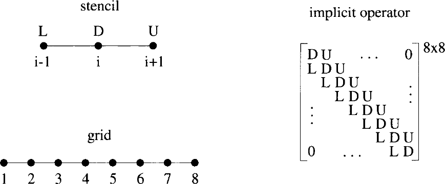
图6.1:一维结构网格及相应的三点模板隐式算子矩阵。图例:左上为模板(stencil)——节点\(L\)(\(i-1\))、\(D\)(\(i\))、\(U\)(\(i+1\));左下为网格(grid)——编号1至8的8个网格节点;右侧为隐式算子——\(8\times 8\)块三对角矩阵ï¼非零块为\(L\)、\(D\)、\(U\)ï¼角落处为0。
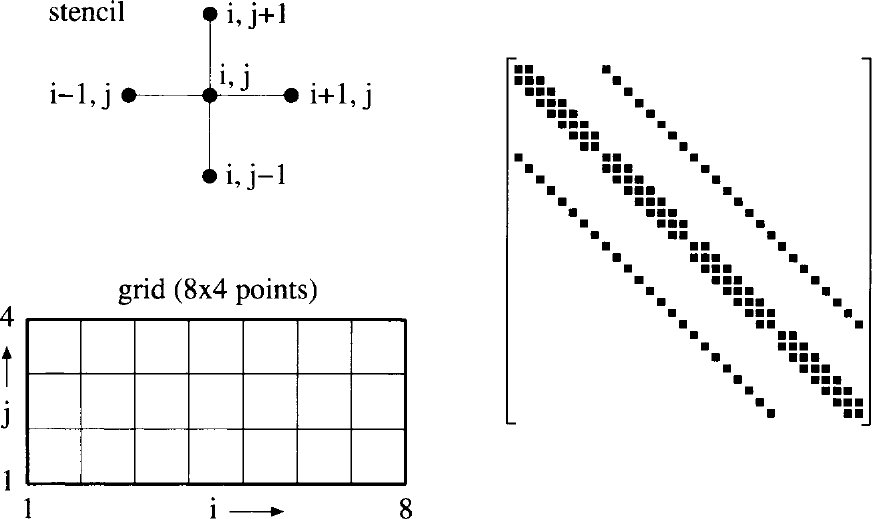
图6.2:二维结构网格(左)及相应的五点模板隐式算子矩阵(右)。图例:模板(stencil)由节点\(i,j\)及其四个邻居\(i-1,j\)、\(i+1,j\)、\(i,j-1\)、\(i,j+1\)组成;网格(grid)为\(8\times 4\)个节点,\(i\)方向编号1至8,\(j\)方向编号1至4;右侧矩阵中非零块矩阵以实心方块表示。
为了将系统矩阵可视化ï¼把隐式算子中与中心节点\(i\)相关联的所有项记为\(\mathbf{D}\)ï¼即en
In order to visualise the system matrix, we denote all terms in the implicit operator associated with the central node \(i\) as \(\mathbf{D}\), i.e.,
把下游节点\((i+1)\)记为\(\mathbf{U}\)ï¼即en
with the downwind node \((i+1)\) as \(\mathbf{U}\), i.e.,
把上游节点\((i-1)\)记为\(\mathbf{L}\)ï¼即en
and with the upwind node \((i-1)\) as \(\mathbf{L}\), i.e.,
对图6.1中网格的全部8个节点写出方程(6.34)ï¼就得到图6.1右侧所示的\(8\times 8\)块三对角矩阵。一维情形下ï¼每个块\(\mathbf{L}\)、\(\mathbf{D}\)和\(\mathbf{U}\)都是一个\(3\times 3\)矩阵(因为有三个守恒方程)。en
respectively. Writing down Eq. (6.34) for all eight nodes of the grid in Fig. 6.1, we obtain the \(8\times 8\) block-tridiagonal matrix displayed on the right side of Fig. 6.1. Each of the blocks \(\mathbf{L}\), \(\mathbf{D}\), and \(\mathbf{U}\) represents a \(3\times 3\) matrix in 1D (because of the three conservation equations).
同样的思想可以推广到多维。例如ï¼若二维空间离散化涉及图6.2所示的五点模板ï¼就会得到块五对角矩阵ï¼如图6.2右侧所示。节点编号时让\(i\)指标比\(j\)指标变化得更快(对应FORTRAN中的\(mat(i,j)\))。应当注意ï¼第二条次对角线与主对角线相距八个元素(即\(i\)方向的节点总数)。最后ï¼如果空间离散化采用图4.9b的七点模板ï¼三维情形的系统矩阵将变为块七对角矩阵。en
The same ideas carry over to multiple dimensions. For example, if the spatial discretisation in 2D would involve the 5-point stencil sketched in Fig. 6.2, we would obtain a block-pentadiagonal matrix. This is shown on the right side of Fig. 6.2. The nodes were ordered such that the \(i\)-index runs faster than the \(j\)-index (corresponds to \(mat(i,j)\) in FORTRAN). It should be noted that the second off-diagonal is at the distance of eight elements from the main diagonal (the total number of nodes in \(i\)-direction). Finally, the system matrix would become block-septadiagonal in 3D, if we would employ the 7-point stencil of Fig. 4.9b for the spatial discretisation.
总之ï¼对结构网格ï¼系统矩阵总是具有规则的、稀疏的带状形式。还应指出ï¼方程(6.28)中的项en
In summary, we can state that the system matrix always possesses a regular, sparse and banded form for structured grids. It should be further mentioned that the term
——它总是位于主对角线上——可能引起困难:当时间步长变大时ï¼某些迭代矩阵求逆格式(如Gauss-Seidel)可能因隐式算子对角占优减弱而失效。en
in Eq. (6.28), which is always located on the main diagonal, can cause difficulties. Namely, if the time step becomes large, some iterative matrix inversion schemes (e.g., Gauss-Seidel) may fail due to reduced diagonal dominance of the implicit operator.
Implicit Operator on Unstructured Grids 非结构网格上的隐式算子
从结构网格过渡到非结构网格时ï¼系统矩阵的外观完全改变。这一点可以借助图6.3所示的小型非结构网格来说明。设空间离散化由5.2.1小节的单元中心格式给出ï¼该格式只使用最近邻单元的流动值(例如像一阶上风格式那样——见5.3.2和5.3.3小节)。于是ï¼例如单元2的模板包括单元18、10和13。所得的系统矩阵显示在图6.3的右侧。显然ï¼由于网格单元(中位对偶格式情形下为节点)一般按任意顺序编号ï¼矩阵不会呈现出规则的模式。只有主对角线——它至少包含表达式(6.35)ï¼可能还包含源项的导数——总是存在。en
The appearance of the system matrix changes completely when we proceed from structured to unstructured grids. This can be demonstrated with the aid of a small unstructured grid sketched in Fig. 6.3. We want assume that the spatial discretisation is given by the cell-centred scheme presented in Subsection 5.2.1, which uses flow values only from the nearest neighbours (e.g., like a first-order upwind scheme - see Subsections 5.3.2 and 5.3.3). Thus, for example, the stencil for cell 2 includes the cells 18, 10, and 13. The resulting system matrix is displayed on the right side of Fig. 6.3. It is obvious that since the grid cells (nodes in the case of a median-dual scheme) are in general numbered in an arbitrary order, no regular pattern can be expected for the matrix. Only the main diagonal, which contains at least the expression (6.35) and possibly the derivative of the source term, is always present.
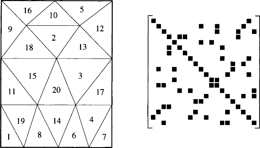
图6.3:二维非结构网格(左)及相应的最近邻模板隐式算子矩阵(右)。图例:左图三角形单元编号1至20;右侧矩阵中非零块矩阵以实心方块表示。
系统矩阵中非零元素的准随机分布是不可取的。它会减慢Gauss-Seidel等迭代求逆方法的收敛速度。此外,ILU(不完全下-上三角分解,Incomplete Lower-Upper)这类Krylov子空间方法的预条件技术也无法高效使用。因此ï¼人们发展了通过对单元(节点)重新编号来大幅减小系统矩阵带宽的策略ï¼即使非零元素聚集到主对角线附近。最著名的重新编号策略是逆Cuthill-McKee(Reverse-Cuthill-McKee,RCM)算法[27]、[28]。图6.4给出了把RCM算法应用于图6.3示例网格后得到的单元编号和系统矩阵。可以看到ï¼矩阵的带宽显著减小ï¼矩阵获得了更规则的结构。en
The quasi-random distribution of nonzero elements in the system matrix is undesirable. It slows down the convergence of iterative inversion methods like Gauss-Seidel. Furthermore, preconditioning techniques for Krylov-subspace methods like ILU (Incomplete Lower-Upper) factorisation scheme cannot be used efficiently. Therefore, strategies were developed where the cells (nodes) are renumbered such that the bandwidth of the system matrix is considerably reduced, i.e., the nonzero elements are clustered close to the main diagonal. The best-known renumbering strategy is the Reverse-Cuthill-McKee (RCM) algorithm [27], [28]. Figure 6.4 shows the resulting cell numbering and the system matrix when the RCM algorithm is applied to the example grid of Fig. 6.3. As we can see, the bandwidth of the matrix is significantly reduced and the matrix obtains a more regular structure.
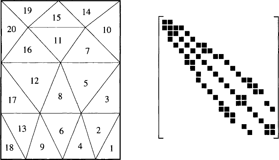
图6.4:用逆Cuthill-McKee(reverse-Cuthill-McKee)排序把图6.3隐式算子的带宽从18减至5。图例:左图为重新编号后的三角形单元网格(编号1至20);右侧矩阵中非零块矩阵以实心方块表示。
为了减少缓存未命中或允许数值格式向量化ï¼还发展了其他一些重新编号策略。综述可参见例如文献[29]。en
Several other renumbering strategies were developed in order to minimise cache misses or to allow for vectorisation of the numerical scheme. An overview can be found, e.g., in Ref. [29].