6.2.4 LU-SGS Scheme LU-SGS格式[cfd-6-2-4]

隐式下-上对称Gauss-Seidel(Lower-Upper Symmetric Gauss-Seidel,LU-SGS)格式ï¼也称为下-上对称逐次超松弛(Lower-Upper Symmetric Successive Overrelaxation,LU-SSOR)格式ï¼因其数值复杂度低、内存需求适中——两者均与显式多级格式相当——而得到广泛使用。此外,LU-SGS格式易于在向量机与并行计算机上实现ï¼既可用于结构网格ï¼也可用于非结构网格。en

The implicit Lower-Upper Symmetric Gauss-Seidel (LU-SGS) scheme, which is also called the Lower-Upper Symmetric Successive Overrelaxation (LU-SSOR) scheme, became widely-used because of its low numerical complexity and modest memory requirements, which are both comparable to an explicit multistage scheme. Furthermore, the LU-SGS scheme can be implemented easily on vector and parallel computers. It can also be used on structured as well as on unstructured grids.

LU-SGS格式源于Jameson与Turkel[49]的工作ï¼他们研究了把隐式算子分解为下、上对角占优因子的方法。LU-SGS方法本身由Yoon与Jameson[50]-[52]提出ï¼作为求解式(6.28)未分解隐式格式的一种松弛方法。Rieger与Jameson[53]进一步发展了该方法并将其应用于三维黏性流场。此后ï¼多位研究者把LU-SGS格式应用于结构网格[54]-[61]与非结构网格[62]-[66]上的黏性流动。LU-SGS方法也常用于化学反应流动的模拟[67]-[71]。en

The LU-SGS scheme has its origins in the work of Jameson and Turkel [49], who considered decompositions of the implicit operator into lower and upper diagonally dominant factors. The LU-SGS method itself was introduced by Yoon and Jameson [50]-[52] as a relaxation method for solving the unfactored implicit scheme in Eq. (6.28). It was further developed and applied to 3-D viscous flow fields by Rieger and Jameson [53]. Since then, various researchers applied the LU-SGS scheme to viscous flows on structured [54]-[61] and on unstructured grids [62]-[66]. The LU-SGS approach is often used for the simulation of chemically reacting flows [67]-[71].

对于式(6.29)中对流通量的线性化,LU-SGS格式采用Steger与Warming(见6.2.2小节)一阶精度通量向量分裂方法的一种简化形式。无论显式算子如何离散ï¼该线性化始终保持不变。此外,LU-SGS格式基于把式(6.28)的隐式算子因式分解为以下三部分en

The LU-SGS scheme employs a simplification of the first-order accurate flux-vector splitting approach due to Steger and Warming (see Subsection 6.2.2) for the linearisation of the convective fluxes in Eq. (6.29). The linearisation is always kept the same regardless of the discretisation of the explicit operator. The LU-SGS scheme is further based on the factorisation of the implicit operator in Eq. (6.28) into the following three parts

\left(\mathbf{D} + \mathbf{L}\right)\mathbf{D}^{-1}\left(\mathbf{D} + \mathbf{U}\right)\Delta\vec{W}^{n} = -\vec{R}^{n}_{I}. \tag{6.49}

这些因子的构造使得 $\mathbf{L}$ 只包含严格下三角矩阵中的项, $\mathbf{U}$ 只包含严格上三角矩阵中的项ï¼而 $\mathbf{D}$ 只包含对角项。值得注意的是ï¼因子的数目始终保持不变ï¼与空间维数无关。en

The factors are constructed such that $\mathbf{L}$ consists only of terms in the strictly lower triangular matrix, $\mathbf{U}$ of terms in the strictly upper triangular matrix and $\mathbf{D}$ of diagonal terms. It is important to remark that the number of factors remains always the same independent of the number of space dimensions.

LU-SGS格式的系统矩阵(式(6.49)))可以分两步求逆——一次前扫与一次后扫ï¼即en

The system matrix of the LU-SGS scheme (Eq. (6.49))) can be inverted in two steps - a forward and a backward sweep, i.e.,

\begin{aligned} \left(\mathbf{D} + \mathbf{L}\right)\Delta\vec{W}^{(1)} &= -\vec{R}^{n}_{I}\\ \left(\mathbf{D} + \mathbf{U}\right)\Delta\vec{W}^{n} &= \mathbf{D}\Delta\vec{W}^{(1)}_{I} \end{aligned} \tag{6.50}

其中 $\vec{W}^{n+1} = \vec{W}^{n} + \Delta\vec{W}^{n}$ 。算子 $\mathbf{L}$ 、 $\mathbf{D}$ 、 $\mathbf{U}$ 以及求逆过程在结构网格与非结构网格上存在若干差异。因此ï¼下面分别讨论这两种情形。en

with $\vec{W}^{n+1} = \vec{W}^{n} + \Delta\vec{W}^{n}$ . The operators $\mathbf{L}$ , $\mathbf{D}$ , and $\mathbf{U}$ and also the inversion procedure differ on structured and unstructured grids in some respects. Therefore, we shall discuss below each case separately.

LU-SGS on Structured Grids 结构网格上的LU-SGS

在结构网格上ï¼算子定义为(参见[50]-[52]以及[68]、[55])en

On structured grids, the operators are defined as (see [50]-[52], and [68], [55])

\begin{aligned} \mathbf{L} &= \left(\bar{A}^{+} + \bar{A}_{v}\right)_{i-1}\Delta S^{I}_{i-1/2} + \left(\bar{A}^{+} + \bar{A}_{v}\right)_{j-1}\Delta S^{J}_{j-1/2}\\ &\quad + \left(\bar{A}^{+} + \bar{A}_{v}\right)_{k-1}\Delta S^{K}_{k-1/2}\\ \mathbf{U} &= \left(\bar{A}^{-} - \bar{A}_{v}\right)_{i+1}\Delta S^{I}_{i+1/2} + \left(\bar{A}^{-} - \bar{A}_{v}\right)_{j+1}\Delta S^{J}_{j+1/2}\\ &\quad + \left(\bar{A}^{-} - \bar{A}_{v}\right)_{k+1}\Delta S^{K}_{k+1/2}\\ \mathbf{D} &= \frac{\Omega}{\Delta t}\bar{I} + \left(\bar{A}^{-} - \bar{A}_{v}\right)\Delta S^{I}_{i-1/2} + \left(\bar{A}^{-} - \bar{A}_{v}\right)\Delta S^{J}_{j-1/2}\\ &\quad + \left(\bar{A}^{-} - \bar{A}_{v}\right)\Delta S^{K}_{k-1/2} + \left(\bar{A}^{+} + \bar{A}_{v}\right)\Delta S^{I}_{i+1/2}\\ &\quad + \left(\bar{A}^{+} + \bar{A}_{v}\right)\Delta S^{J}_{j+1/2} + \left(\bar{A}^{+} + \bar{A}_{v}\right)\Delta S^{K}_{k+1/2} - \frac{\partial(\Omega\vec{Q})}{\partial\vec{W}}. \end{aligned} \tag{6.51}

为了便于阅读ï¼式(6.51)中只标出了与 $$i$$ 、 $$j$$ 、 $$k$$ 不同的那些节点指标(单元中心格式下为单元指标)。 $\Delta S$ 上的上标 $$i$$ 、 $$j$$ 、 $$k$$ 指示计算空间中的方向。正/负通量雅可比 $\bar{A}^{\pm}$ 以及黏性通量雅可比 $\bar{A}_{v}$ 中的单位法向量ï¼与相关联的面面积 $\Delta S$ 一样ï¼在控制体的同一侧取值。注意ï¼这里假定单位法向量指向控制体外侧。相反ï¼在各种文献中则假定控制体相对两侧的单位法向量指向同一方向。en

For better readability, only those node indices (or cell indices in the case of a cell-centred scheme) are shown in Eq. (6.51), which differ from $$i, j, k$$ . The superscripts $$i, j, k$$ at $\Delta S$ indicate the direction in the computational space. The unit normal vectors in the positive/negative flux Jacobians $\bar{A}^{\pm}$ and in the viscous flux Jacobians $\bar{A}_{v}$ are evaluated at the same side of the control volume like the associated face areas $\Delta S$ . Note that the unit normal vectors are assumed to point outwards of the control volume. In contrast, in various references it is supposed that the unit normal vectors from opposite sides of the control volume point in the same direction.

式(6.51)中的黏性通量雅可比要么数值计算ï¼要么按式(6.45)用其TSL近似代替。无论边界层的实际取向如何ï¼都可以在所有计算坐标上应用TSL近似。进一步的简化是把黏性通量雅可比用黏性谱半径(式(6.19))代替ï¼即 $\bar{A}_{v}\Delta S \approx \hat{\Lambda}_{v}$ ï¼如文献[63]所建议。en

The viscous flux Jacobians in Eq. (6.51) are either computed numerically, or are replaced by their TSL approximation, corresponding to Eq. (6.45). It is possible to apply the TSL approximation in all computational coordinates, regardless of the actual orientation of the boundary layer(s). A further simplification consists of substituting the viscous flux Jacobians by the viscous spectral radii (Eq. (6.19)), i.e., $\bar{A}_{v}\Delta S \approx \hat{\Lambda}_{v}$ , as suggested in [63].

分裂的对流通量雅可比 $\bar{A}^{\pm}$ 的构造方式是:(+)矩阵的特征值全部非负,(-)矩阵的特征值全部非正。一般地ï¼这些矩阵定义为[49]en

The split convective flux Jacobians $\bar{A}^{\pm}$ are constructed in such a way that the eigenvalues of the (+) matrices are all non-negative, and of the (-) matrices are all non-positive. In general, the matrices are defined as [49]

\bar{A}^{\pm}\Delta S = \frac{1}{2}\left(\bar{A}_{c}\Delta S \pm r_{A}\bar{I}\right), \quad r_{A} = \omega\hat{\Lambda}_{c}, \tag{6.52}

其中 $\bar{A}_{c}$ 为对流通量雅可比(见A.9节), $\hat{\Lambda}_{c}$ 为对流通量雅可比的谱半径(由式(4.53)或式(6.15)给出)。当忽略 $\bar{A}_{c}$ 的导数时ï¼上述近似(6.52)与式(6.40)相似。式(6.52)中的因子 $\omega$ 为超松弛参数ï¼它同时决定隐式耗散的量ï¼从而影响格式的收敛特性。该因子可在 $1 < \omega \le 2$ 范围内选取。 $\omega$ 值越高,LU-SGS格式的稳定性越好ï¼但可能减慢到定态的收敛。式(6.52)中雅可比 $\bar{A}^{\pm}$ 的定义保证了系统矩阵对角占优ï¼这对迭代求逆过程(6.50)的效率与稳健性非常重要。en

where $\bar{A}_{c}$ stands for the convective flux Jacobian (Section A.9) and $\hat{\Lambda}_{c}$ represents the spectral radius of the convective flux Jacobian (given by Eq. (4.53) or Eq. (6.15)), respectively. Note the similarity between the above approximation (6.52) and Eq. (6.40), when the derivatives of $\bar{A}_{c}$ are neglected. The factor $\omega$ in Eq. (6.52) represents an overrelaxation parameter. It also determines the amount of implicit dissipation and hence influences the convergence properties of the scheme. The factor can be chosen in the range $1 < \omega \le 2$ . Higher values of $\omega$ increase the stability of the LU-SGS scheme, but may slow down the convergence to steady state. The definition of the Jacobians $\bar{A}^{\pm}$ in Eq. (6.52) ensures a diagonally dominant system matrix, which is very important for the efficiency and robustness of the iterative inversion procedure (6.50).

按式(6.52)的分裂ï¼再结合平均后的面向量ï¼可简化对角算子 $\mathbf{D}$ 的计算en

The splitting according to Eq. (6.52) together with averaged face vectors allow a simplified evaluation of the diagonal operator $\mathbf{D}$

\begin{aligned} \mathbf{D} &= \left[\frac{\Omega}{\Delta t} + \omega\left(\hat{\Lambda}^{I}_{c} + \hat{\Lambda}^{J}_{c} + \hat{\Lambda}^{K}_{c}\right)\right]\bar{I}\\ &\quad + 2\left(\bar{A}^{I}_{v}\Delta S^{I} + \bar{A}^{J}_{v}\Delta S^{J} + \bar{A}^{K}_{v}\Delta S^{K}\right) - \frac{\partial(\Omega\vec{Q})}{\partial\vec{W}}. \end{aligned} \tag{6.53}

对流通量雅可比的谱半径 $\hat{\Lambda}_{c}$ 由式(6.15)给出。面面积与法向量分别按式(6.16)在I、J或K方向上作平均。正如马上将看到的ï¼这一近似有助于显著减少运算量与内存需求。en

The spectral radii of the convective flux Jacobians $\hat{\Lambda}_{c}$ are given in Eq. (6.15). The face areas and normal vectors are averaged in the respective I-, J-, or K-direction according to Eq. (6.16). As we shall see immediately, this approximation helps to reduce the operation count and the memory requirements significantly.

LU-SGS方法的一个显著特点在于式(6.50)中前扫与后扫的执行方式。在二维中ï¼扫掠沿计算空间中的对角线 $(i+j) = \mathrm{const.}$ 进行。图6.5描绘了前扫(式(6.50)第一行)的情形。这样, $\mathbf{L}$ 算子与 $\mathbf{U}$ 算子所涉及的非对角项便可以从扫掠的前一部分获得(在图6.5中用叉号表示)。在三维中ï¼隐式算子在 $i+j+k = \mathrm{const.}$ 平面上求逆ï¼如图6.6所示意。于是,LU-SGS格式可以写为en

A distinguishing feature of the LU-SGS method is how the forward and the backward sweep in Eq. (6.50) are carried out. In 2D, the sweeps are accomplished along diagonal lines $(i+j) = \mathrm{const.}$ in computational space. This is depicted in Fig. 6.5 for the forward sweep (first line of Eq. (6.50))). In this way, the off-diagonal terms involved in the $\mathbf{L}$ and the $\mathbf{U}$ operator become known from the previous part of a sweep (denoted by crosses in Fig. 6.5). In 3D, the implicit operator is inverted on $i+j+k = \mathrm{const.}$ planes, as sketched in Fig. 6.6. Hence, the LU-SGS scheme can be written as

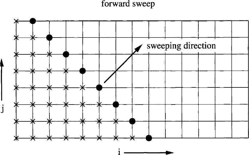
\begin{aligned} \mathbf{D}\Delta\vec{W}^{(1)}_{i,j,k} &= -\vec{R}^{n}_{i,j,k} - \mathbf{L}\Delta\vec{W}^{(1)}\\ \mathbf{D}\Delta\vec{W}^{n}_{i,j,k} &= \mathbf{D}\Delta\vec{W}^{(1)}_{i,j,k} - \mathbf{U}\Delta\vec{W}^{n}. \end{aligned} \tag{6.54}

图6.5:LU-SGS格式在计算空间中的扫掠方向

图6.5:LU-SGS格式在计算空间中的扫掠方向。图例: $\bullet$ 表示算子 $\mathbf{D}$ 当前被求逆的位置(直线 $i+j=\mathrm{const.}$ ); $\times$ 表示 $\mathbf{L}$ 的已更新值。

图6.6:三维隐式LU-SGS格式扫掠的对角面

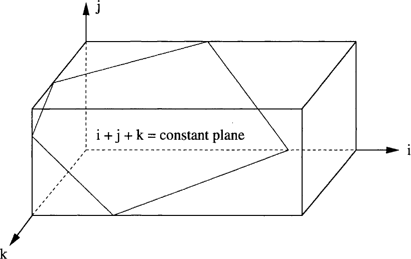
图6.6:三维隐式LU-SGS格式扫掠的对角面。图内标注: $$i+j+k$$ =常数平面(i+j+k = constant plane)。

由式(6.54)可见ï¼唯一需要求逆的是对角项 $\mathbf{D}$ 。这样,LU-SGS方法把稀疏带状矩阵的求逆转化为块对角矩阵的求逆。此外ï¼若式(6.53)中的黏性通量雅可比用黏性谱半径近似ï¼算子 $\mathbf{D}$ 便成为对角矩阵(源项除外)。因此ï¼与其他隐式格式(例如前面讨论过的ADI格式)相比,LU-SGS格式所需的计算量非常小。而且ï¼对角算子的求逆可以对角面上的每个节点(单元)独立进行ï¼这使该格式易于向量化。对角面上节点/单元的指标可用如下伪代码获得[72]:en

As we can see from Eq. (6.54), the only term which needs to be inverted is the diagonal term $\mathbf{D}$ . Thus, the LU-SGS methodology transforms the inversion of a sparse banded matrix into the inversion of a block-diagonal matrix. Furthermore, if the viscous flux Jacobians in Eq. (6.53) are approximated by the viscous spectral radii, the operator $\mathbf{D}$ becomes a diagonal matrix (except for the source term). Hence, the LU-SGS scheme requires a very small computational effort as compared to other implicit schemes (e.g., the ADI scheme discussed previously). Furthermore, the inversion of the diagonal operator can be carried out independently for each node (cell) of the diagonal plane, which makes the scheme easy to vectorise. The indices of the nodes/cells on the diagonal planes can be obtained with the following pseudo-code [72]:

    DO plane = 1, nplanes
       DO k = 1, kmax
          DO j = 1, jmax
             DO i = 1, imax
                IF (i+j+k = plane+2) store indices
             ENDDO
          ENDDO
       ENDDO
    ENDDO

对角面的数目为:nplanes = imax + jmax + kmax - 2。显然ï¼为了获得更高的计算效率ï¼可对上述代码进行优化。en

The number of diagonal planes is: nplanes = imax + jmax + kmax - 2. Obviously, the above code can be optimised for higher computational efficiency.

为了避免在 $\mathbf{L}$ 与 $\mathbf{U}$ 中显式计算并存储对流通量雅可比ï¼乘积 $\bar{A}^{\pm}\Delta\vec{W}^{n}$ 可以用通量的Taylor级数展开代替[53]。利用式(6.52)ï¼可以写出en

In order to avoid explicit evaluation and storage of the convective flux Jacobians in $\mathbf{L}$ and $\mathbf{U}$ , the products $\bar{A}^{\pm}\Delta\vec{W}^{n}$ can be substituted by Taylor series expansion of the fluxes [53]. Using Eq. (6.52), we can write

\left(\bar{A}^{\pm}\Delta S\right)\Delta\vec{W}^{n} \approx \frac{1}{2}\left(\Delta\vec{F}_{c}\Delta S \pm r_{A}\bar{I}\Delta\vec{W}^{n}\right) \tag{6.55}

其中对流通量的更新为en

with the update of the convective fluxes

\Delta\vec{F}_{c} = \vec{F}^{n+1}_{c} - \vec{F}^{n}_{c}. \tag{6.56}

由于是沿对角面扫掠, $\vec{F}^{n+1}_{c}$ 此时已知ï¼式(6.55)给出的简化才成为可能。这使LU-SGS格式的数值工作量进一步显著下降。en

The simplification given by Eq. (6.55) is possible due to the sweeping along diagonal planes, since $\vec{F}^{n+1}_{c}$ is then known. This leads to a further significant decrease of the numerical effort of the LU-SGS scheme.

时间步长 $\Delta t$ 可以按6.1.4小节所述方法、用式(6.14)计算。但应注意ï¼如Rieger与Jameson[53]所述ï¼当 $\Delta t \to \infty$ 时ï¼式(6.49)的隐式LU-SGS格式代表一次近似Newton迭代。因此ï¼实践中对定常流动一般使用 $10^{4}$ 到 $10^{6}$ 量级的CFL数。此时收敛由超松弛参数 $\omega$ 控制。对于非定常流动的模拟ï¼可以采用下文6.3节给出的形式;另一种可能是使用文献[73]所述的LU-SGS格式的修正版本。en

The time step $\Delta t$ can be computed in the same way as presented in Subsection 6.1.4, using Eq. (6.14). However, it should be noted that the implicit LU-SGS scheme in Eq. (6.49) represents an approximate Newton iteration in the case of $\Delta t \to \infty$ as stated by Rieger and Jameson [53]. Thus in general, CFL numbers of the order of $10^{4}$ to $10^{6}$ are used in practice for stationary flows. The convergence is then controlled by the overrelaxation parameter $\omega$ . For the simulation of unsteady flows, we may employ the formulation presented below in Section 6.3. Another possibility is to use the modified version of the LU-SGS scheme described in Ref. [73].

LU-SGS on Unstructured Grids 非结构网格上的LU-SGS

这里ï¼对中位对偶(median-dual)格式ï¼算子为[63]-[65]en

Here, the operators read for a median-dual scheme [63]-[65]

\begin{aligned} \mathbf{L} &= \sum_{j\in L(i)}\left[\bar{A}^{+}_{j} + \left(\bar{A}_{v}\right)_{j}\right]\Delta S_{ij}\\ \mathbf{U} &= \sum_{j\in U(i)}\left[\bar{A}^{-}_{j} - \left(\bar{A}_{v}\right)_{j}\right]\Delta S_{ij}\\ \mathbf{D} &= \frac{\Omega_{i}}{\Delta t_{i}}\bar{I} + \frac{\omega}{2}\left(\hat{\Lambda}_{c}\right)_{i} + \sum_{j=1}^{N_{F}}\left(\bar{A}_{v}\right)_{i}\Delta S_{ij} - \frac{\partial(\Omega_{i}\vec{Q}_{i})}{\partial\vec{W}}. \end{aligned} \tag{6.57}

在式(6.57)中, $$L(i)$$ 与 $$U(i)$$ 表示属于下(上)矩阵的节点 $$i$$ 的最近邻节点, $\Delta S_{ij}$ 表示与边 $$ij$$ 相关联的面面积(见图5.9), $N_{F}$ 表示控制体 $\Omega_{i}$ 的面数。对流通量的谱半径 $(\hat{\Lambda}_{c})_{i}$ 由式(6.21)计算。黏性通量雅可比 $\bar{A}_{v}$ 同样可以用其谱半径近似[63]。此时ï¼对角算子变为en

In Eq. (6.57), $$L(i)$$ , and $$U(i)$$ denote the nearest neighbours of node $$i$$ which belong to the lower (upper) matrix, $\Delta S_{ij}$ represents the face area associated with the edge $$ij$$ (see Fig. 5.9), and $N_{F}$ stands for the number of faces of the control volume $\Omega_{i}$ , respectively. The spectral radius of the convective fluxes $(\hat{\Lambda}_{c})_{i}$ is computed by Eq. (6.21). The viscous flux Jacobian $\bar{A}_{v}$ can be again approximated by its spectral radius [63]. In this case, the diagonal operator becomes

\mathbf{D} = \frac{\Omega_{i}}{\Delta t_{i}}\bar{I} + \frac{\omega}{2}\left(\hat{\Lambda}_{c}\right)_{i} + \left(\hat{\Lambda}_{v}\right)_{i} - \frac{\partial(\Omega_{i}\vec{Q}_{i})}{\partial\vec{W}}, \tag{6.58}

其中 $(\hat{\Lambda}_{v})_{i}$ 按式(6.21)计算。对单元中心格式ï¼可以得到与式(6.57)、(6.58)类似的公式ï¼主要区别是 $\mathbf{L}$ 与 $\mathbf{U}$ 算子中的求和遍及单元的各个面而非相邻边。en

where $(\hat{\Lambda}_{v})_{i}$ is evaluated according to Eq. (6.21). Formulae similar to Eq. (6.57) and (6.58) can be obtained in the case of the cell-centred scheme. The major difference is that the summation in the $\mathbf{L}$ and the $\mathbf{U}$ operator is conducted over faces of the cell instead of incident edges.

式(6.57)中的集合 $$L(i)$$ 与 $$U(i)$$ 应起到与结构网格上对角面相同的作用。为此ï¼必须把节点(单元)划分为层ï¼使得[63]:

当前层的节点 $$i$$ (单元 $$I$$ )与流动变量已更新的层相连——否则LU-SGS格式退化为Jacobi迭代;
同一层内的节点(单元)彼此不相连——否则该格式无法向量化。

The sets $$L(i)$$ and $$U(i)$$ in Eq. (6.57) should fulfil the same function as the diagonal planes on structured grids. For this reason, it is necessary to arrange the nodes (cells) into layers such that [63]:

nodes $$i$$ (cells $$I$$ ) of a current layer have connections to layers with previously updated flow variables - otherwise the LU-SGS scheme degenerates to a Jacobi iteration,
nodes (cells) in a layer are not connected to each other - otherwise the scheme could not be vectorised.

对中位对偶格式ï¼可按文献[63]所述的方法生成分层;单元中心格式的做法见于[74]、[75]。en

The layers can be generated for the median-dual scheme with a procedure described in Ref. [63]. Approaches for the cell-centred scheme were suggested in [74], [75].

恰当定义集合 $$L(i)$$ 与 $$U(i)$$ 后ï¼可实现如下两步求逆过程[63]-[65]en

An appropriate definition of the sets $$L(i)$$ and $$U(i)$$ allows for the following two-step inversion procedure [63]-[65]

\begin{aligned} \mathbf{D}\Delta\vec{W}^{(1)}_{i} &= -\vec{R}^{n}_{i} - \sum_{j\in L(i)}\frac{1}{2}\left[\left(\Delta F^{(1)}_{c}\right)_{j}\Delta S_{ij} + \left(r^{*}_{A}\right)_{j}\bar{I}\Delta\vec{W}^{(1)}_{j}\right]\\ \mathbf{D}\Delta\vec{W}^{n}_{i} &= \mathbf{D}\Delta\vec{W}^{(1)}_{i} - \sum_{j\in U(i)}\frac{1}{2}\left[\left(\Delta F^{n}_{c}\right)_{j}\Delta S_{ij} - \left(r^{*}_{A}\right)_{j}\bar{I}\Delta\vec{W}^{n}_{j}\right], \end{aligned} \tag{6.59}

其中黏性雅可比用其谱半径近似ï¼正/负雅可比按式(6.55)线性化。此外ï¼因子 $(r^{*}_{A})_{j}$ 定义为en

where the viscous Jacobians were approximated by their spectral radii and where the positive/negative Jacobians were linearised according to Eq. (6.55). Furthermore, the factor $(r^{*}_{A})_{j}$ is defined as

\begin{aligned} \left(r^{*}_{A}\right)_{j} &= \omega\left(\left|\vec{v}_{j}\cdot\vec{n}_{ij}\right| + c_{j}\right)\Delta S_{ij}\\ &\quad + \frac{\Delta S_{i,j}}{\left\|\vec{r}_{j} - \vec{r}_{i}\right\|_{2}}\left[\max\left(\frac{4}{3\rho_{j}}, \frac{\gamma_{j}}{\rho_{j}}\right)\left(\frac{\mu_{L}}{Pr_{L}} + \frac{\mu_{T}}{Pr_{T}}\right)_{j}\right] \end{aligned} \tag{6.60}

其中 $\|\vec{r}_{j} - \vec{r}_{i}\|_{2}$ 为边 $$ij$$ 的长度。en

with $\|\vec{r}_{j} - \vec{r}_{i}\|_{2}$ being the length of the edge $$ij$$ .

时间步长可按显式格式(式(6.20)))同样方式计算。但应略去黏性特征值ï¼因为黏性项已包含在隐式算子中ï¼不会像显式格式那样减小时间步长。对定常流动,CFL数可在 $10^{4}$ 到 $10^{6}$ 范围内选取。随后可用超松弛参数 $\omega$ 来调节LU-SGS格式的收敛速度与稳健性。en

The time step can be computed in the same way as for the explicit scheme (Eq. (6.20))). However, the viscous eigenvalue should be omitted, since the viscous terms are already contained in the implicit operator and hence do not reduce the time step as in the case of an explicit scheme. The CFL number can be chosen in the range from $10^{4}$ to $10^{6}$ for steady flows. The convergence speed and the robustness of the LU-SGS scheme can then be tuned using the overrelaxation parameter $\omega$ .