9.4.3 Implementation on Structured Grids 结构网格上的实现[cfd-9-4-3]
多重网格在结构网格上的实现很简单,因为粗网格可以很容易地通过在相应坐标方向上每隔一条删除一条网格线来生成,网格线间距因此为\(2h\)、\(4h\)等。这保证了粗网格上的数值工作量相对于最细网格保持在较低水平。若干代表性例子见文献[11]-[13]、[20]-[22]、[26]、[32]-[36]。en
The implementation of multigrid on structured grids is straightforward since the coarse grids can be easily generated by deleting every second grid line in the respective coordinate direction. The spacing of the grid lines is therefore \(2h\), \(4h\), etc. This guarantees that the numerical effort on the coarse grids stays low as compared to the finest grid. Several representative examples are provided in Refs. [11]-[13], [20]-[22], [26], [32]-[36].
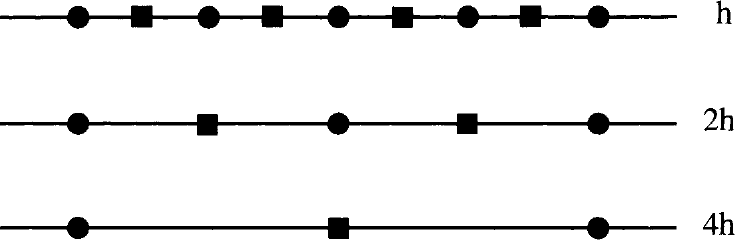
图9.5:细网格(h)与两个粗网格(2h、4h)的一维表示。圆圈表示网格点,矩形表示单元中心。
从图9.5可以得出,解插值算子、残差限制算子和修正延拓算子在单元中心(cell-centred)格式与节点中心(cell-vertex,顶点)格式下必须有不同的定义。例如,相邻两层网格每隔一个网格点就有一个公共点;相反,单元中心的位置总是彼此错开的。因此,下面将分别针对单元中心和节点中心(与顶点格式相同)两种有限体积格式讨论转移算子的标准形式。en
As we can conclude from Fig. 9.5, the operators for the solution interpolation, the restriction of residuals and the prolongation of corrections have to be defined differently for cell-centred and node-centred (cell-vertex) schemes. For example, two successive grids have every second grid point in common. On the contrary, the cell centres are always at different locations. Therefore, we shall discuss the standard forms of the transfer operators separately for the cell-centred and node-centred (identical to cell-vertex) finite-volume schemes.
除了下面将要介绍的对称的、纯几何定义的限制与延拓算子之外,文献[16]第4章还提出了偏上风的形式。计及流动方程特征的上风限制与延拓可以提高多重网格格式在高超声速流动中的鲁棒性。为节省篇幅,下面只针对节点中心空间离散讨论上风延拓算子的实现。en
Apart from the symmetrical, purely geometrically defined restriction and prolongation operators, which will be presented next, upwind-biased forms were suggested in [16], Chapter 4. Upwind restriction and prolongation, which account both for the characteristics of the flow equations, improve the robustness of the multigrid scheme for hypersonic flows. In order to save space, we shall discuss the implementation of an upwind prolongation operator for the node-centred spatial discretisation only.
Transfer Operators for the Cell-Centred Scheme 单元中心格式的转移算子
三维情形采用类似的转移算子,此时求和遍及构成一个粗网格单元的八个细网格控制体。en
Similar transfer operator is employed in 3D, where the summation is over the eight fine-grid control volumes, which form one coarse-grid cell.
限制算子定义为包含在一个粗网格控制体内的所有单元的残差之和。因此,二维情形为(参见图9.6a)en
The restriction operator is defined as a sum of the residuals from all cells which are contained in one coarse-grid control volume. Hence, in 2D we have (cf. Fig. 9.6a)
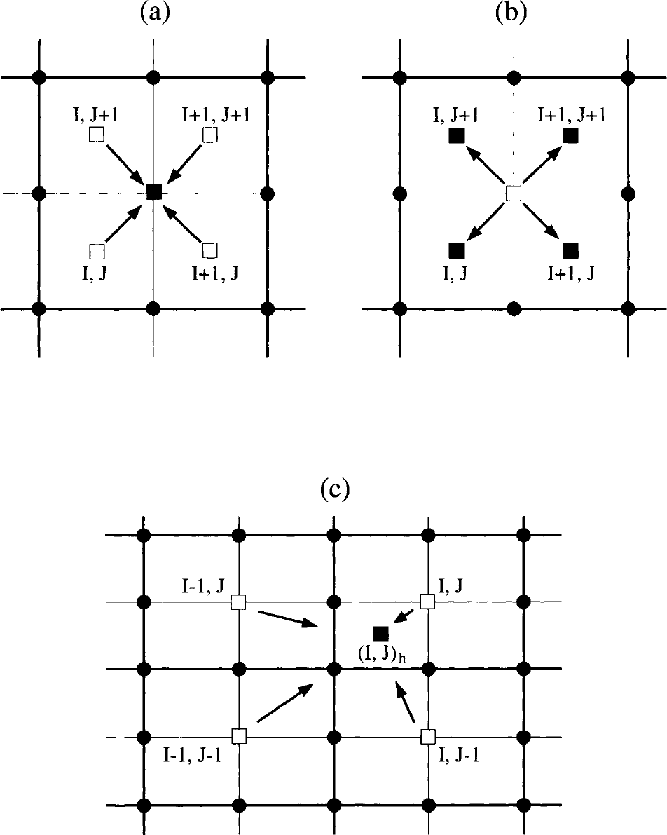
图9.6:二维结构网格单元中心格式的解插值与残差限制(a),粗网格修正的延拓(b、c)。实心圆=网格点;实心矩形=插值目标单元中心;矩形=插值来源单元中心;粗线=粗网格;细线=细网格。
粗网格修正即式(9.23)的延拓可以用两种不同的方式进行。第一种方式:如果把\(\delta\vec{W}_{2h}\)平均分配给周围所有单元中心(如图9.6b所示),就得到零阶延拓算子。例如en
The prolongation of the coarse-grid correction Eq. (9.23) can be conducted in two different ways. First, a zeroth-order prolongation operator results, if \(\delta\vec{W}_{2h}\) is equally distributed to all surrounding cell centres as indicated in Fig. 9.6b. Thus, for instance
第二种方式能使多重网格格式收敛更快,它分两步进行。第一步,把\(\delta\vec{W}_{2h}\)插值到网格节点上,做法与顶点格式相同(见下文)。第二步,对节点值取平均,得到细网格单元中心的值。参照图9.6c,可以推导出如下最终关系式en
The second possibility, which leads to a faster convergence of the multigrid scheme, consists of two steps. In a first step, \(\delta\vec{W}_{2h}\) is interpolated to the grid nodes like for the cell-vertex scheme (see below). In a second step, the nodal values are averaged to obtain the value in the centre of the fine-grid cell. Referring to Fig. 9.6c, the following final relationship can be derived
三维情形的对应表达式可以通过类似的过程得到,为en
The corresponding expression in 3D can be found by a similar procedure. It reads
Transfer Operators for the Cell-Vertex Scheme 顶点格式的转移算子
由于细网格与粗网格拥有公共节点,解可以简单地通过直接注入(injection)来转移,即en
Because of the common nodes between the fine and coarse grid, the solution can be transfered simply by injection, i.e.,
标准的中心限制算子是对构成一个粗网格单元的四个(三维为八个)细网格单元的所有节点作线性插值。按照图9.7,二维情形的限制残差计算为en
The standard central restriction operator represents a linear interpolation from the nodes of all four (eight in 3D) fine-grid cells, which resemble one coarse-grid cell. According to Fig. 9.7, the restricted residual is computed in 2D as
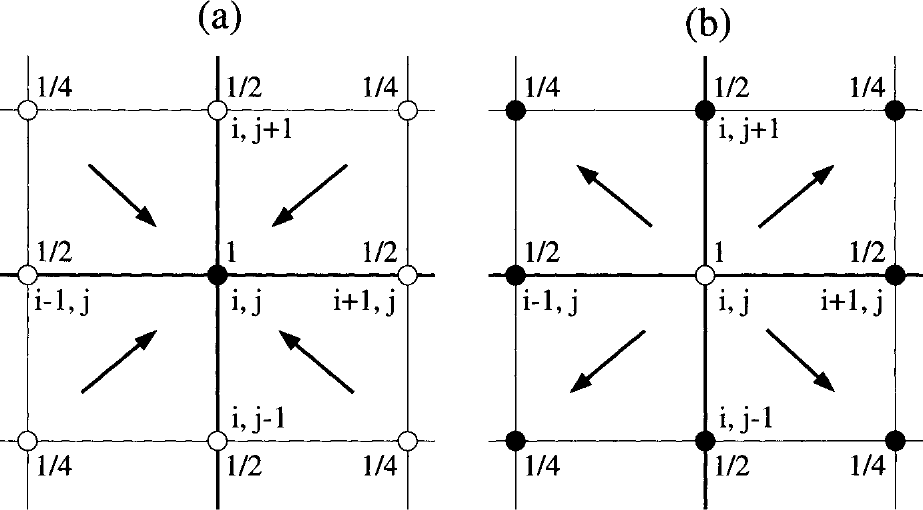
图9.7:二维结构网格顶点格式的限制(a)与延拓(b)的插值系数。实心圆=插值目标点;圆圈=插值来源点;粗线=粗网格;细线=细网格。点(i, j)为两网格共有。
三维情形,细网格残差按下式收集en
In 3D, the fine-grid residuals are collected as follows
其中各因子为en
with the factors
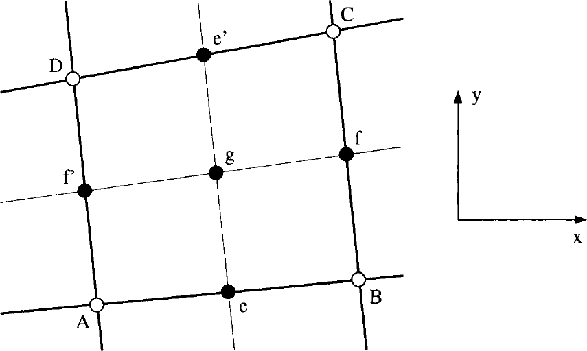
图9.8:二维上风延拓。点A、B、C、D为粗网格(粗线)与细网格共有;点e、f、e′、f′、g仅属于细网格(细线)。
式(9.34)中只标出了与\(i, j, k\)不同的那些下标。需要注意的是,在限制之前必须先把所有物理边界点和虚单元点上的残差\(\vec{R}^{n+1}_{h}\)置为零。en
In the above Eq. (9.34), only those indices are shown which are different from \(i, j, k\). It should be noted that the residuals \(\vec{R}^{n+1}_{h}\) must be set to zero at all physical boundary and dummy points before the restriction.
粗网格修正的延拓可以实现对粗网格点的循环:在循环内,把值\((\delta\vec{W}_{2h})_{i,j,k}\)用与限制相同的权重分配到细网格点上(参见图9.7b),并把各部分贡献累加起来,从而得到细网格每一点上完整的转移修正量。en
The prolongation of the coarse-grid correction can be implemented as a loop over the points of the coarse grid. Within the loop, the values \((\delta\vec{W}_{2h})_{i,j,k}\) are distributed to the fine-grid points using the same weights as for the restriction (cf. Fig. 9.7b). The particular contributions are summed up in order to obtain the complete transfered correction at each point of the fine grid.
Upwind Prolongation (Cell-Vertex Scheme) 上风延拓(顶点格式)
原则上,上风延拓既可以在特征变量中表述,也可以在守恒变量中表述。文献[16]提出了一种特别高效的守恒变量实现。该方法根据马赫数和速度方向对式(9.23)中的修正作偏上风插值。其数值代价非常低,但对于高马赫数流动却能显著改善多重网格格式的鲁棒性[16]。en
In principle, upwind prolongation can be formulated either in characteristic or in conservative variables. A particularly efficient implementation in conservative variables was proposed in [16]. The methodology employs upwind-biased interpolation of the corrections in Eq. (9.23) according to the Mach number and the velocity direction. The numerical effort is very low, nevertheless the robustness of the multigrid scheme can be significantly improved for high Mach-number flows [16].
把解修正\(\delta\vec{W}_{2h}\)插值到较细网格分两步完成。第一步,把两网格共有的点\(A\)、\(B\)、\(C\)、\(D\)(见图9.8)处的修正直接转移到较细网格。第二步,把修正插值到仅存在于较细网格上的点\(e\)、\(f\)、\(e'\)、\(f'\)和\(g\)。插值取决于相应点马赫数的符号和绝对值。这里的马赫数用逆变速度计算en
The interpolation of the solution corrections \(\delta\vec{W}_{2h}\) to the finer grid is accomplished in two steps. In the first step, the corrections at the points \(A\), \(B\), \(C\), and \(D\) (see Fig. 9.8), which are common to both grids, are transferred directly to the finer grid. In the second step, the corrections are interpolated to the points \(e\), \(f\), \(e'\), \(f'\) and \(g\), which are contained only on the finer grid. The interpolation depends on the sign and the absolute value of the Mach number at the corresponding point. The Mach number in this case is calculated using
式(9.35)中的法向向量\(\vec{n}\)既可以由控制体面向量平均得到(沿\(A-B\)方向),也可以由点\(A\)到点\(B\)的向量归一化得到。然后,按如下规则把修正转移到点\(e\)en
is employed. The normal vector \(\vec{n}\) in Eq. (9.35) can be obtained either by averaging the face vectors of the control volume (in the direction \(A-B\)), or by normalising the vector from point \(A\) to point \(B\). Then, the correction is transferred to point \(e\) according to the rule
同样的过程也适用于点\(f\)到\(f'\)。上风处理有助于使网格间的信息交换更好地与真实物理相匹配。往点\(g\)的插值则更困难。文献[16]中只是简单地对周围点\(A\)到\(D\)的值取平均en
The same procedure applies also to the points \(f\) to \(f'\). The upwinding helps to match the information exchange between the grids better to the real physics. The interpolation to the point \(g\) is more difficult. In Ref. [16], the values at the surrounding points \(A\) to \(D\) were simply averaged
不过,某种上风加权插值会更合适。上风延拓也可以在三维中以类似方式实现。尽管作了简化,仍在多个测试算例中得到了令人鼓舞的结果[16]。en
However, some sort of upwind weighted interpolation would be more appropriate. The upwind prolongation can be implemented in similar way also in 3D. Despite the simplification, encouraging results were obtained in a number of test cases [16].