9.4 Multigrid 多重网格[cfd-9-4]
多重网格(multigrid)方法是一种非常强大的加速技术(参见图3.7)。它基于在一系列逐级加粗的网格上求解控制方程,然后把粗网格上的解更新组合起来,加到最细网格的解上。该技术最初由Brandt[19]为椭圆型偏微分方程而发展,随后由Jameson[20]-[22]应用于欧拉方程。此后,多重网格格式又被用于求解Navier-Stokes方程[11]-[13]、[23]-[31]。多重网格方法既可以结合显式时间推进格式实现,也可以结合隐式时间推进格式实现[32]-[36]。当前研究的目标是显著提高多重网格对双曲型流动问题的效率[37]-[40]。en
The multigrid methodology is a very powerful acceleration technique (cf. Fig. 3.7). It is based on the solution of the governing equations on a series of successively coarser grids. The solution updates from the coarse grid are then combined and added to the solution on the finest grid. The technique was originally developed by Brandt [19] for elliptic partial differential equations and later applied to the Euler equations by Jameson [20]-[22]. After that, the multigrid scheme was employed to solve the Navier-Stokes equations [11]-[13], [23]-[31]. The multigrid method can be implemented for both the explicit and the implicit time-stepping schemes [32]-[36]. The goal of the current research is the significant improvement of the efficiency of multigrid for hyperbolic flow problems [37]-[40].
多重网格格式的基本思想是利用粗网格,使最细网格上的解更快地趋于定常态。为此利用了两种效应:
- 1. 在较粗的网格上可以采用较大的时间步长(因为控制体更大),同时数值工作量也更小。由于求新解的工作主要分布在较粗的网格上,因此收敛更快,计算时间也得以减少。
- 2. 大多数显式和隐式时间推进格式与迭代格式主要能有效削减解误差的高频分量(见10.3节)。低频分量通常很难被阻尼。在初始阶段(最大误差被消除的阶段)过后,这会导致向定常态收敛缓慢。多重网格格式正是在这一点上发挥作用——最细网格上的低频分量在较粗网格上变成高频分量,从而被逐级阻尼掉。其结果是,整个误差被非常迅速地削减,收敛显著加速。
en
The basic idea of the multigrid scheme is to employ coarse grids in order to drive the solution on the finest grid faster to steady-state. Two effects are utilised for this purpose:
- 1. larger time steps can be employed on the coarser grids (owing to a larger control volume) in conjunction with a reduced numerical effort. Since the work for determining a new solution is distributed mainly over the coarser grids, a more rapid convergence and a reduction of the computing time results.
- 2. The majority of the explicit and implicit time-stepping and iterative schemes reduces efficiently mainly the high-frequency components of the solution error (see Section 10.3). The low-frequency components are usually only hardly damped. This results in a slow convergence to the steady state, after the initial phase (where the largest errors are eliminated) is over. The multigrid scheme helps at this point - the low-frequency components on the finest grid becomes high-frequency components on the coarser grids and are successively damped. As a result, the entire error is very quickly reduced, and the convergence is significantly accelerated.
因此可以看到,多重网格格式的成败在很大程度上取决于时间推进格式或迭代格式能否良好地阻尼高频误差分量。en
Thus, as we can see, the success of the multigrid scheme depends heavily on good damping of the high-frequency error components by the time-stepping or iterative scheme.
几何多重网格之外的一种替代方法是代数多重网格(Algebraic Multigrid,AMG)方法[41]-[48]。AMG技术为隐式格式而发展,它直接作用于系统矩阵(即左端算子)。AMG的基本思想是应用一个粗化矩阵来降低隐式算子的维数,从而减少方程的数目。随后求解这个代表粗层的约化系统,以获得细层解的修正。粗化矩阵的构造方式是把耦合最强(即系统矩阵中非对角元最大)的方程相加在一起。这样,粗层的生成完全由流动问题的物理特性决定,而与网格无关。因此,AMG的优点是无需构造或存储粗网格拓扑,这在复杂的非结构网格上尤其有利。en
An alternative to the geometrical multigrid is provided by the Algebraic Multigrid (AMG) method [41]-[48]. The AMG technique was developed for implicit schemes, where it operates directly on the system matrix (the left-hand side operator). The basic idea of AMG is to apply a coarsening matrix in order to reduce the dimension of the implicit operator and hence the number of equations. The reduced system, which represents a coarse level, is then solved to obtain the correction of the fine-level solution. The coarsening matrix is constructed such that the equations with the strongest coupling (i.e., the largest off-diagonals in the system matrix) are added together. Thus, the generation of coarse levels is governed solely by the physics of the flow problem and not by the grid. Therefore, the advantage of AMG is that no coarse grid topology has to be constructed or stored, which is particularly beneficial on complex unstructured grids.
9.4.1 Basic Multigrid Cycle 基本多重网格循环[cfd-9-4-1]
在应用几何多重网格格式之前,必须先生成较粗的网格。标准做法是在所有坐标方向上均匀地粗化网格。不过,Mulder[49]提出了一种称为半粗化(semicoarsening)的方法。此时网格只在一个方向上粗化,且该方向从一个粗层到另一个粗层轮换。半粗化方法特别适合控制方程在某一空间方向上呈刚性的流动问题,边界层中垂直于壁面的方向即为一例。将半粗化应用于Navier-Stokes方程的工作见文献[26]、[50]、[51]。en
Before the geometric multigrid scheme can be applied, the coarser grids have to be generated. The standard way is to coarsen the grid evenly in all coordinate directions. However, Mulder [49] proposed an approach called semicoarsening. Here, the grid is coarsened only in one direction, which is changed from one coarse level to another. The semicoarsening methodology is especially suited for flow problems, where the governing equations are stiff in one spatial direction. An example is the direction normal to the wall in boundary layers. Applications of semicoarsening to the Navier-Stokes equations were reported, e.g., in Refs. [26], [50], [51].
按照关系式(6.1),细网格上离散化的控制方程为en
The discretised governing equations on the fine grid read in accordance with the relationship (6.1)
以下用下标\(h\)表示最细网格,该记号源于网格线的间距(在非结构网格上为控制体的特征尺寸)。从已知解\(\vec{W}^{n}_{h}\)出发,用某个合适的迭代格式经过一个时间步后得到新解\(\vec{W}^{n+1}_{h}\),并用这个解计算新的残差\(\vec{R}^{n+1}_{h}\)。为了利用粗网格改进解\(\vec{W}^{n+1}_{h}\),需要进行以下三个步骤:en
In the following, the finest grid will be denoted by subscript \(h\) in reference to the spacing of the grid lines (characteristic dimension of the control volume on unstructured grids). Starting from a known solution \(\vec{W}^{n}_{h}\), a new solution \(\vec{W}^{n+1}_{h}\) is obtained after one time step with some suitable iterative scheme. A new residual \(\vec{R}^{n+1}_{h}\) is evaluated with this solution. In order to improve the solution \(\vec{W}^{n+1}_{h}\) using a coarse grid, the following three steps are carried out:
1. Transfer of the Solution and Residuals to the Coarser Grid 1. 把解与残差转移到较粗网格
解通过插值转移到粗网格上en
The solution is transferred to the coarse grid by means of the interpolation
其中下标\(2h\)表示粗网格¹,\(\hat{I}^{2h}_{h}\)为插值算子(interpolation operator)。残差也必须转移到粗网格上,以便对其低频误差分量进行光顺。为此采用守恒的转移算子,这意味着当控制体尺寸增大时,残差的值必须增大相同的数量。此外还需要细网格的残差,以便在粗网格上保持细网格解的精度。为此,构造一个源项,即所谓的强迫函数(forcing function)[19]、[22],它等于由细网格转移来的残差与用初始解\(\vec{W}^{(0)}_{2h}\)(式(9.17))在粗网格上计算出的残差之差,即en
where the subscript \(2h\) denotes the coarse grid¹ and \(\hat{I}^{2h}_{h}\) is the interpolation operator. The residuals have to be transferred to the coarse grid as well, so that their low-frequency error components can be smoothed. A conservative transfer operator is employed for this purpose. This means that when the control volume size increases, the value of the residual must increase by the same amount. The residuals of the fine grid are also required in order to retain the solution accuracy of the fine grid on the coarse grid. For this purpose, a source term, the so-called forcing function [19], [22], is formed as the difference between the residual transferred from the fine grid and the residual computed using the initial solution \(\vec{W}^{(0)}_{2h}\) (Eq. (9.17)) on the coarse grid, i.e,
¹原书脚注:The notation 2h must not be understood in a strictly geometric sense. On unstructured grids, the ratio of the characteristic dimensions of the control volumes on the fine and the coarse grid will usually differ from two. The same holds also for semicoarsening.(记号2h不应按严格的几何意义理解。在非结构网格上,细网格与粗网格上控制体特征尺寸之比通常并不等于2。半粗化的情形也是如此。)
这里\(I^{2h}_{h}\)表示把残差从细网格转移到粗网格的限制算子(restriction operator)。这类多重网格格式称为完全近似存储(Full Approximation Storage,FAS)方法[19]。FAS方法特别适合非线性方程,因为系统中的非线性通过重新离散化被带到粗层。en
Here, \(I^{2h}_{h}\) represents the restriction operator which transfers residuals from the fine to the coarse grid. This type of multigrid scheme is known as the Full Approximation Storage (FAS) method [19]. The FAS method is particularly suited for non-linear equations because the nonlinearities in the system are carried down to the coarse levels through the re-discretisation.
2. Calculation of a New Solution on the Coarse Grid 2. 在粗网格上计算新解
于是,时间推进格式可以写成en
Hence, the time-stepping scheme can be written in the form
对于显式多级格式(6.1.1小节),这就导致en
In the case of the explicit multistage scheme (Subsection 6.1.1), this results in
这与式(6.5)一致。需要注意的是,在第一次迭代(式(9.21)中的级)时,\((\vec{R}_F)_{2h}\)与从细网格转移来的残差完全相同(即式(9.18)中的\((\vec{R}_F)_{2h} = I^{2h}_{h}\vec{R}^{n+1}_{h}\))。这保证了粗网格上的解依赖于细网格的残差,从而保持细网格的精度。en
in accordance with Eq. (6.5). It has to be noted that during the first iteration (stage in Eq. (9.21)), \((\vec{R}_F)_{2h}\) is identical to the residual transferred from the fine grid (i.e., \((\vec{R}_F)_{2h} = I^{2h}_{h}\vec{R}^{n+1}_{h}\) from Eq. (9.18)). This guarantees that the solution on the coarse grid depends on the residual of the fine grid and thus retains the accuracy of the fine grid.
粗网格上空间离散格式的精度是一个重要问题。由于粗网格不影响细网格解的精度,一阶格式就足够了。与高阶格式相比,粗网格上一阶精度离散的优点是鲁棒性更强、阻尼特性更好、数值工作量更低。en
An important question is the accuracy of the spatial discretisation scheme on coarse grids. Since the coarse grids do not influence the accuracy of the fine-grid solution, first-order schemes are sufficient. The advantages of first-order accurate discretisation on coarse grids are the increased robustness, better damping properties, and lower numerical effort in comparison to higher-order schemes.
3. Solution Interpolation from the Coarse to the Fine Grid 3. 解由粗网格插值回细网格
在粗网格上进行一个或多个时间步(迭代)之后,计算相对于初始——插值——解(式(9.17))的修正量。这个所谓的粗网格修正(coarse grid correction)由下式给出en
After one or several time steps (iterations) were carried out on the coarse grid, the correction with respect to the initial - interpolated - solution (Eq. (9.17)) is computed. This so-called coarse grid correction is given by
粗网格修正被插值回细网格,以改进那里的解。于是,细网格上的新解为en
The coarse-grid correction is interpolated to the fine grid in order to improve the solution there. Hence, the new solution on the fine grid reads
其中\(I^{h}_{2h}\)称为延拓算子(prolongation operator)。en
where \(I^{h}_{2h}\) is denoted as the prolongation operator.
9.4.2 Multigrid Strategies 多重网格策略[cfd-9-4-2]
上面描述的基本多重网格格式只含一个粗网格。如果存在多个粗网格,则重复步骤1和步骤2,直到到达最粗网格。重要的是要认识到,粗网格上的强迫函数是由式(9.19)限制后的修正残差构成的。例如,在粗网格\(4h\)上,强迫函数由下式得到en
The basic multigrid scheme described above consists of one coarse grid only. If multiple coarse grids are present, steps 1 and 2 are repeated until the coarsest grid is reached. It is important to realize that the forcing function on the coarse grids is formed from the restricted corrected residual of Eq. (9.19)). For example, on the coarse grid \(4h\), the forcing function is obtained from
这样,最细网格的残差控制着所有粗网格上解的精度。在最粗网格上进行给定数目的时间步之后,可以逐层重复步骤3,直到再次到达最细网格。这一过程称为锯齿形循环或V循环(见图9.4a)。不过,也可以在粗网格上执行更多的循环。这种策略称为W循环,如图9.4b所示。它在跨声速流动中采用得尤其频繁。而对于超声速和高超声速流动,V循环被证明效率更高。en
In this way, the residual of the finest grid controls the accuracy of the solution on all coarse grids. After a given number of time steps on the coarsest grid, step 3 can be successively repeated until the finest grid is reached again. This procedure is known as a saw-tooth or V-cycle (see Fig. 9.4a). However, it is also possible to conduct more cycles on the coarse grids. This strategy, termed the W-cycle, is displayed in Fig. 9.4b. It is employed particularly frequently for transonic flows. In the case of supersonic and hypersonic flows, the V-cycle proved to be more efficient.
Number of Time Steps 时间步数
限制前和延拓后的最优时间步数取决于时间推进格式的类型。对于显式多级格式(6.1.1或6.1.2小节),通常在残差限制之前只进行一个时间步,延拓之后不进行时间步。不过,把粗网格修正(式(9.22))在加到细网格解\(\vec{W}^{n+1}_{h}\)(式(9.23))上之前先做光顺,可以改进多重网格格式的鲁棒性。这里采用与9.3节相同的中心隐式光顺(系数取为常数)。en
The optimum number of time steps before the restriction and after the prolongation depends on the type of the time-stepping scheme. In the case of the explicit multistage scheme (Subsection 6.1.1 or 6.1.2), it is common to carry out only one time step before the restriction of residuals and no time step after the prolongation. However, the robustness of the multigrid scheme can be improved by smoothing the coarse grid corrections (Eq. (9.22)) before adding them to the fine grid solution \(\vec{W}^{n+1}_{h}\) (Eq. (9.23)). The same central implicit smoothing (with constant coefficients) as described in Section 9.3 is utilised.
另一种常用的时间推进方法——隐式LU-SGS格式(见6.2.4小节)——为了获得最佳多重网格效率,需要在限制之前进行两次迭代[34]。延拓之后的时间步数则取决于空间离散。对于中心格式(4.3.1小节),不需要时间步[34]-[36],但可以对解修正进行光顺。相反,如果采用上风空间离散,则应在延拓之后进行一个时间步。实践证明,这种(2,1)策略在各种流动条件下的鲁棒性和计算时间方面都是最优的[35]、[36]。en
The other popular time-stepping method, the implicit LU-SGS scheme (see Subsection 6.2.4), requires two iterations before the restriction for the best multigrid efficiency [34]. The number of time steps after the prolongation depends on the spatial discretisation. In the case of the central scheme (Subsection 4.3.1), no time step is necessary [34]-[36], but the solution correction can be smoothed. On the contrary, one time step should carried out after the prolongation if an upwind spatial discretisation is used. This (2,1)-strategy proved to be an optimum with respect to robustness and computing time for various flow conditions [35], [36].
Starting Grid 起始网格
需要指出的是,实际中多重网格格式并不是直接从最细网格开始的。相反,先从某个粗网格开始执行若干个多重网格循环,把近似解插值到下一层较细的网格(采用与延拓相同的算子),再执行几个循环,然后把解再次插值到下一层更细的网格,如此继续,直到最细网格。这样,只需适度的数值工作量,就能在最细网格上获得一个良好的起始解。这一非常高效的过程称为完全多重网格(Full Multigrid,FMG)方法[19]。en
It should be pointed out that in practice the multigrid scheme is not started directly from the finest grid. Instead, several multigrid cycles are executed from one of the coarse grids. The approximate solution is interpolated to the next finer grid (using the same operator as for the prolongation), few more cycles are performed, the solution is again interpolated to the next finer grid and so on, until the finest grid is reached. In this way, a good starting solution is obtained on the finest grid with only a moderate numerical effort. This very efficient procedure is termed the Full Multigrid (FMG) method [19].
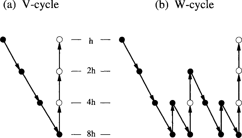
图9.4:多重网格循环的类型。图内标注:(a)V-cycle——V循环;(b)W-cycle——W循环;h、2h、4h、8h——网格层(由细到粗);●——限制前的时间步;∘——延拓后的时间步。
Accuracy of Transfer Operators 转移算子的精度
其中\(m_R\)和\(m_P\)分别表示限制算子和延拓算子能够精确插值的多项式的“次数加1”。例如,线性插值时\(m_R\)或\(m_P\)等于2。此外,\(m_E\)表示控制方程的阶数。因此,欧拉方程的\(m_E = 1\),Navier-Stokes方程的\(m_E = 2\)。如果违反条件(9.25),限制和/或延拓引入的额外误差将干扰细网格解,这样的多重网格格式将收敛得非常缓慢,甚至发散。en
where \(m_R\) and \(m_P\) denote the degree plus 1 of the polynomial, which is exactly interpolated by the restriction and the prolongation operator, respectively. For example, \(m_R\) or \(m_P\) are equal to two in the case of linear interpolation. Furthermore, \(m_E\) represents the order of the governing equations. Thus, \(m_E = 1\) for the Euler equations, and \(m_E = 2\) in the case of the Navier-Stokes equations. If the condition (9.25) is violated, the additional errors introduced by the restriction and/or prolongation will disturb the fine-grid solution. Hence, such multigrid scheme will converge only slowly or it will even diverge.
9.4.3 Implementation on Structured Grids 结构网格上的实现[cfd-9-4-3]
多重网格在结构网格上的实现很简单,因为粗网格可以很容易地通过在相应坐标方向上每隔一条删除一条网格线来生成,网格线间距因此为\(2h\)、\(4h\)等。这保证了粗网格上的数值工作量相对于最细网格保持在较低水平。若干代表性例子见文献[11]-[13]、[20]-[22]、[26]、[32]-[36]。en
The implementation of multigrid on structured grids is straightforward since the coarse grids can be easily generated by deleting every second grid line in the respective coordinate direction. The spacing of the grid lines is therefore \(2h\), \(4h\), etc. This guarantees that the numerical effort on the coarse grids stays low as compared to the finest grid. Several representative examples are provided in Refs. [11]-[13], [20]-[22], [26], [32]-[36].
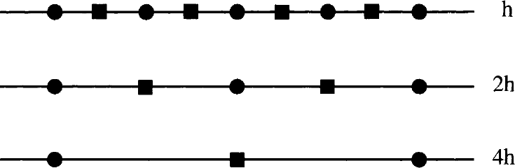
图9.5:细网格(h)与两个粗网格(2h、4h)的一维表示。圆圈表示网格点,矩形表示单元中心。
从图9.5可以得出,解插值算子、残差限制算子和修正延拓算子在单元中心(cell-centred)格式与节点中心(cell-vertex,顶点)格式下必须有不同的定义。例如,相邻两层网格每隔一个网格点就有一个公共点;相反,单元中心的位置总是彼此错开的。因此,下面将分别针对单元中心和节点中心(与顶点格式相同)两种有限体积格式讨论转移算子的标准形式。en
As we can conclude from Fig. 9.5, the operators for the solution interpolation, the restriction of residuals and the prolongation of corrections have to be defined differently for cell-centred and node-centred (cell-vertex) schemes. For example, two successive grids have every second grid point in common. On the contrary, the cell centres are always at different locations. Therefore, we shall discuss the standard forms of the transfer operators separately for the cell-centred and node-centred (identical to cell-vertex) finite-volume schemes.
除了下面将要介绍的对称的、纯几何定义的限制与延拓算子之外,文献[16]第4章还提出了偏上风的形式。计及流动方程特征的上风限制与延拓可以提高多重网格格式在高超声速流动中的鲁棒性。为节省篇幅,下面只针对节点中心空间离散讨论上风延拓算子的实现。en
Apart from the symmetrical, purely geometrically defined restriction and prolongation operators, which will be presented next, upwind-biased forms were suggested in [16], Chapter 4. Upwind restriction and prolongation, which account both for the characteristics of the flow equations, improve the robustness of the multigrid scheme for hypersonic flows. In order to save space, we shall discuss the implementation of an upwind prolongation operator for the node-centred spatial discretisation only.
Transfer Operators for the Cell-Centred Scheme 单元中心格式的转移算子
三维情形采用类似的转移算子,此时求和遍及构成一个粗网格单元的八个细网格控制体。en
Similar transfer operator is employed in 3D, where the summation is over the eight fine-grid control volumes, which form one coarse-grid cell.
限制算子定义为包含在一个粗网格控制体内的所有单元的残差之和。因此,二维情形为(参见图9.6a)en
The restriction operator is defined as a sum of the residuals from all cells which are contained in one coarse-grid control volume. Hence, in 2D we have (cf. Fig. 9.6a)
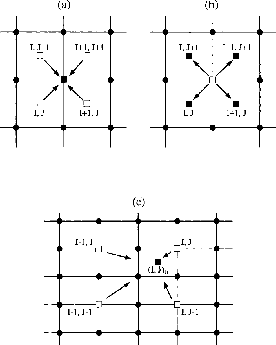
图9.6:二维结构网格单元中心格式的解插值与残差限制(a),粗网格修正的延拓(b、c)。实心圆=网格点;实心矩形=插值目标单元中心;矩形=插值来源单元中心;粗线=粗网格;细线=细网格。
粗网格修正即式(9.23)的延拓可以用两种不同的方式进行。第一种方式:如果把\(\delta\vec{W}_{2h}\)平均分配给周围所有单元中心(如图9.6b所示),就得到零阶延拓算子。例如en
The prolongation of the coarse-grid correction Eq. (9.23) can be conducted in two different ways. First, a zeroth-order prolongation operator results, if \(\delta\vec{W}_{2h}\) is equally distributed to all surrounding cell centres as indicated in Fig. 9.6b. Thus, for instance
第二种方式能使多重网格格式收敛更快,它分两步进行。第一步,把\(\delta\vec{W}_{2h}\)插值到网格节点上,做法与顶点格式相同(见下文)。第二步,对节点值取平均,得到细网格单元中心的值。参照图9.6c,可以推导出如下最终关系式en
The second possibility, which leads to a faster convergence of the multigrid scheme, consists of two steps. In a first step, \(\delta\vec{W}_{2h}\) is interpolated to the grid nodes like for the cell-vertex scheme (see below). In a second step, the nodal values are averaged to obtain the value in the centre of the fine-grid cell. Referring to Fig. 9.6c, the following final relationship can be derived
三维情形的对应表达式可以通过类似的过程得到,为en
The corresponding expression in 3D can be found by a similar procedure. It reads
Transfer Operators for the Cell-Vertex Scheme 顶点格式的转移算子
由于细网格与粗网格拥有公共节点,解可以简单地通过直接注入(injection)来转移,即en
Because of the common nodes between the fine and coarse grid, the solution can be transfered simply by injection, i.e.,
标准的中心限制算子是对构成一个粗网格单元的四个(三维为八个)细网格单元的所有节点作线性插值。按照图9.7,二维情形的限制残差计算为en
The standard central restriction operator represents a linear interpolation from the nodes of all four (eight in 3D) fine-grid cells, which resemble one coarse-grid cell. According to Fig. 9.7, the restricted residual is computed in 2D as
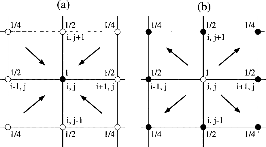
图9.7:二维结构网格顶点格式的限制(a)与延拓(b)的插值系数。实心圆=插值目标点;圆圈=插值来源点;粗线=粗网格;细线=细网格。点(i, j)为两网格共有。
三维情形,细网格残差按下式收集en
In 3D, the fine-grid residuals are collected as follows
其中各因子为en
with the factors
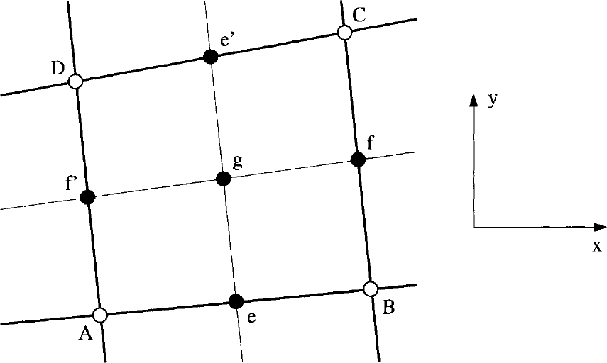
图9.8:二维上风延拓。点A、B、C、D为粗网格(粗线)与细网格共有;点e、f、e′、f′、g仅属于细网格(细线)。
式(9.34)中只标出了与\(i, j, k\)不同的那些下标。需要注意的是,在限制之前必须先把所有物理边界点和虚单元点上的残差\(\vec{R}^{n+1}_{h}\)置为零。en
In the above Eq. (9.34), only those indices are shown which are different from \(i, j, k\). It should be noted that the residuals \(\vec{R}^{n+1}_{h}\) must be set to zero at all physical boundary and dummy points before the restriction.
粗网格修正的延拓可以实现对粗网格点的循环:在循环内,把值\((\delta\vec{W}_{2h})_{i,j,k}\)用与限制相同的权重分配到细网格点上(参见图9.7b),并把各部分贡献累加起来,从而得到细网格每一点上完整的转移修正量。en
The prolongation of the coarse-grid correction can be implemented as a loop over the points of the coarse grid. Within the loop, the values \((\delta\vec{W}_{2h})_{i,j,k}\) are distributed to the fine-grid points using the same weights as for the restriction (cf. Fig. 9.7b). The particular contributions are summed up in order to obtain the complete transfered correction at each point of the fine grid.
Upwind Prolongation (Cell-Vertex Scheme) 上风延拓(顶点格式)
原则上,上风延拓既可以在特征变量中表述,也可以在守恒变量中表述。文献[16]提出了一种特别高效的守恒变量实现。该方法根据马赫数和速度方向对式(9.23)中的修正作偏上风插值。其数值代价非常低,但对于高马赫数流动却能显著改善多重网格格式的鲁棒性[16]。en
In principle, upwind prolongation can be formulated either in characteristic or in conservative variables. A particularly efficient implementation in conservative variables was proposed in [16]. The methodology employs upwind-biased interpolation of the corrections in Eq. (9.23) according to the Mach number and the velocity direction. The numerical effort is very low, nevertheless the robustness of the multigrid scheme can be significantly improved for high Mach-number flows [16].
把解修正\(\delta\vec{W}_{2h}\)插值到较细网格分两步完成。第一步,把两网格共有的点\(A\)、\(B\)、\(C\)、\(D\)(见图9.8)处的修正直接转移到较细网格。第二步,把修正插值到仅存在于较细网格上的点\(e\)、\(f\)、\(e'\)、\(f'\)和\(g\)。插值取决于相应点马赫数的符号和绝对值。这里的马赫数用逆变速度计算en
The interpolation of the solution corrections \(\delta\vec{W}_{2h}\) to the finer grid is accomplished in two steps. In the first step, the corrections at the points \(A\), \(B\), \(C\), and \(D\) (see Fig. 9.8), which are common to both grids, are transferred directly to the finer grid. In the second step, the corrections are interpolated to the points \(e\), \(f\), \(e'\), \(f'\) and \(g\), which are contained only on the finer grid. The interpolation depends on the sign and the absolute value of the Mach number at the corresponding point. The Mach number in this case is calculated using
式(9.35)中的法向向量\(\vec{n}\)既可以由控制体面向量平均得到(沿\(A-B\)方向),也可以由点\(A\)到点\(B\)的向量归一化得到。然后,按如下规则把修正转移到点\(e\)en
is employed. The normal vector \(\vec{n}\) in Eq. (9.35) can be obtained either by averaging the face vectors of the control volume (in the direction \(A-B\)), or by normalising the vector from point \(A\) to point \(B\). Then, the correction is transferred to point \(e\) according to the rule
同样的过程也适用于点\(f\)到\(f'\)。上风处理有助于使网格间的信息交换更好地与真实物理相匹配。往点\(g\)的插值则更困难。文献[16]中只是简单地对周围点\(A\)到\(D\)的值取平均en
The same procedure applies also to the points \(f\) to \(f'\). The upwinding helps to match the information exchange between the grids better to the real physics. The interpolation to the point \(g\) is more difficult. In Ref. [16], the values at the surrounding points \(A\) to \(D\) were simply averaged
不过,某种上风加权插值会更合适。上风延拓也可以在三维中以类似方式实现。尽管作了简化,仍在多个测试算例中得到了令人鼓舞的结果[16]。en
However, some sort of upwind weighted interpolation would be more appropriate. The upwind prolongation can be implemented in similar way also in 3D. Despite the simplification, encouraging results were obtained in a number of test cases [16].
9.4.4 Implementation on Unstructured Grids 非结构网格上的实现[cfd-9-4-4]
与结构网格相比,非结构网格情形下粗网格的构造要复杂得多。问题在于如何从一组没有任何特定排序的单元(网格单元)出发,构造出均匀粗化的网格。此外,粗网格与细网格的单元体积之比也必须保持在一定的范围内(二维约为4,三维约为8)。解决该问题的一种可能途径是采用AMG方法[41]-[48],我们在9.4节开头已简要讨论过。不过,几何多重网格目前仍使用得更广泛,因此这里集中讨论这一方法。en
As compared to the structured grids, the construction of the coarse grids is much more involved in the case of unstructured grids. The problem is how to construct an uniformly coarsened grid from a set of elements (grid cells) which have no particular ordering. Additionally, the ratio of the cell volumes of the coarse to the fine grid has to stay within a certain margins (about 4 in 2D and 8 in 3D). One possibility how to solve this problem is to apply the AMG methodology [41]-[48], which we briefly discussed at the beginning of Section 9.4. However, the geometric multigrid is still more widely used. Therefore, we shall concentrate here on this approach.
粗网格的生成主要有三类方法:
- 非嵌套网格(nonnested-grids)方法;
- 拓扑方法;
- 控制体聚合。
对上述方法的综述见文献[53]和[54]。en
Three main methods for the generation of coarse grids can be identified:
- nonnested-grids approach,
- topological methods, and
- agglomeration of control volumes.
Reviews of the above methods were presented in Refs. [53] and [54].
标准的限制与延拓算子基于纯几何定义的插值。Leclerq和Stoufflet[55]提出了上风转移算子,对含强激波的流动尤其有前景。他们的上风限制/延拓先把残差/修正变换到特征变量,作偏上风插值之后,再把限制/延拓后的值变换回物理变量。文献[16]给出了一种数值代价低得多的上风多重网格方法(另见9.4.3小节式(9.36))。en
The standard restriction and prolongation operators are based on purely geometrically defined interpolation. Leclerq and Stoufflet [55] suggested upwind transfer operators, which are particularly promising for flows with strong shocks. Their upwind restriction/prolongation is based on the transformation of the residuals/corrections into the characteristic variables. After an upwind-biased interpolation, the restricted/prolongated values are transformed back into the physical variables. Numerically much less expensive upwind multigrid method was presented in Ref. [16] (see also Subsection 9.4.3, Eq. (9.36)).
Nonnested Grids 非嵌套网格
最直观的想法是生成一系列完全独立的、逐级加粗的网格[56]-[61]。这些网格不必含有任何公共节点,因此称为非嵌套网格(nonnested grids)。然而,重要的几何特征(前后缘、机身头部等)必须在所有粗网格上保留下来,这在几何外形复杂时并不容易做到。如今基于非嵌套网格的多重网格已很少使用。en
The most obvious idea is to generate a sequence of completely independent, increasingly coarser grids [56]-[61]. It is not necessary that the grids contain any common nodes. Therefore, we speak of nonnested grids. However, it is important that the main geometrical features (leading and trailing edge, fuselage nose, etc.) are retained on all coarse grids. This is not easy to accomplish, particularly in the case of a geometrically complex configuration. Multigrid based on nonnested grids is hardly used today.
Topological Methods 拓扑方法
一种具体的做法是应用基于图的算法从细网格中删除某些节点,然后对剩余节点重新三角化[62]、[63]。与非嵌套网格方法相反,由于相邻网格含有公共节点,网格间的插值变得更容易。但在几何贴合性方面,该方法继承了非嵌套网格的缺点。en
One particular approach applies graph-based algorithms in order to remove certain nodes from the fine grid. The remaining nodes are then re-triangulated [62], [63]. On the contrary to the nonnested-grids approach, the interpolation between the grids becomes easier, since the successive grids contain common nodes. However, the method inherits the drawback of the nonnested grids with respect to geometry conformance.
另一种拓扑方法采用网格加密(grid refinement)[64]、[29]、[65]:从粗网格出发,通过单元剖分生成更细的网格。该方法既可以在整个物理域上应用,也可以只在局部(如边界层处)应用。其缺点是最细网格的质量强烈依赖于初始粗网格和加密过程。这个问题可以部分地通过边交换(edge swapping)[66]、[67]来缓解。en
A further topological method employs grid refinement [64], [29], [65]. The technique starts from a coarse grid and generates finer grids by element division. The methodology can be applied either over the whole physical domain or only locally (e.g., at boundary layers). The disadvantage of this approach is that the quality of the finest grid strongly depends on the initial coarse grid and the refinement procedure. The problem can be partially cured by edge swapping [66], [67].
生成粗网格的另一个想法基于边收缩(edge collapsing)[68]。它最初是为四面体网格上的无黏流动发展的,后来在文献[69]中被推广到混合单元网格上的黏性流动。en
Another idea for the generation of coarse grids is based on edge collapsing [68]. It was initially developed for inviscid flows on tetrahedral grids. The edge-collapsing method was further extended to viscous flows on mixed-element grids in [69].
Agglomeration Multigrid Method 聚合多重网格方法
非结构网格上一种非常高效的方法是所谓的聚合多重网格(agglomeration multigrid)。它最早由Lallemand[70]、Lallemand等[71]以及Koobus等[72]提出。后来,多位作者采用了聚合多重网格[73]-[77]、[31]。该方法通过把细网格的控制体与其邻居融合来生成粗网格,得到的粗网格由逐级增大的、形状不规则的多面体单元组成,如图9.9所示。可以看到,聚合技术完整保留了边界表面的离散,这是它相对于前面讨论的所有非结构多重网格方法的一个显著优点。不过应当指出,迄今为止聚合多重网格的实现大多基于中位对偶顶点格式(median-dual cell-vertex scheme,5.2.2小节)。聚合多重网格在单元中心格式(5.2.1小节)上的应用见文献[73]。en
A very efficient methodology for unstructured grids is the so-called agglomeration multigrid. It was first presented by Lallemand [70], Lallemand et al. [71] and by Koobus et al. [72]. Later on, the agglomeration multigrid was adopted by various authors [73]-[77], [31]. The method generates a coarse grid by fusing the control volumes of the finer grid with their neighbours. The resulting coarse grids consist of successively larger, irregularly shaped polyhedral cells. This is depicted in Fig. 9.9. As we can see, the agglomeration technique retains the full discretisation of the boundary surfaces. This represents a significant advantage over all previously discussed unstructured multigrid methods. However, it should be mentioned that up to now, implementations of the agglomeration multigrid were based mostly on the median-dual cell-vertex scheme (Subsection 5.2.2). The application of the agglomeration multigrid to a cell-centred scheme (Subsection 5.2.1) was described in [73].
Generation of Coarse Grids by Volume Agglomeration 体积聚合生成粗网格
节点中心格式的体积聚合按以下步骤进行:
- 1. 建立所谓的种子点(seed points)列表。种子点是被选中用来聚合周围控制体的网格点。种子点列表既可以包含那些构成近似极大独立集[75]的点,也可以简单地包含当前网格层的全部点。
- 2. 遍历所有种子点。
- 3. 如果该种子点尚未聚合,则聚合其所有尚未聚合的最近邻(由一条边相连)。
- 4. 检查粗化比(即一个粗网格控制体内包含多少个细网格控制体)。如果粗化比小于4(三维为8),则把已聚合最近邻的邻居(若未关联到其他种子点)加入进来,直至达到最优粗化比。文献[27]提出优先聚合那些至少与两个(三维为三个)已聚合最近邻相连的距离为2的邻居。
- 5. 如果列表中仍有种子点,转到步骤2。
- 6. 消除单例(singletons)。单例是指因没有未聚合的邻居而未能被聚合的孤立控制体。把单例与粗化比最小的相邻控制体聚合,即可将其消除。这样得到的粗网格层,其控制体面积的分布更加规则[31]。
en
The volume agglomeration for a node-centred scheme proceeds in the following steps:
- 1. build a list of the so-called seed points. Seed points are grid points selected to agglomerate the surrounding control volumes. The list of seed points can contain either those points which form an approximate maximal independent set [75], or simply all points of the current grid level.
- 2. Loop over all seed points.
- 3. If the seed point is unagglomerated, agglomerate all its nearest neighbours (connected by an edge), which were not already agglomerated.
- 4. Check the coarsening ratio (i.e., how many fine-grid control volumes are contained within a coarse-grid volume). If the ratio is less than four (eight in 3D), the neighbours of the already agglomerated nearest neighbours are added (if not associated with another seed point), until the optimum coarsening ratio is achieved. In Ref. [27], it was proposed to agglomerate those distance-two neighbours first, which are connected to at least two (three in 3D) agglomerated nearest neighbours.
- 5. If there are still seed points in the list, goto step 2.
- 6. Eliminate singletons. These are single control volumes which could not be agglomerated, because there were no unagglomerated neighbours. A singleton can be eliminated by agglomeration with such neighbouring control volume, which has the smallest coarsening ratio. This leads to coarse-grid levels with a more regular distribution of control-volume areas [31].
重复上述过程,直到所有粗网格都生成完毕。en
The above procedure is repeated until all coarse grids are generated.
为了保持网格的各向同性,体积聚合必须从边界开始。在三维情形,可能需要用户根据边界的形状指定聚合方向。为克服这一困难,Okamoto等[77]提出了另一种称为全局粗化(global coarsening)的算法。该方法采用基于边着色(edge colouring)的全局剖分方案;剖分方案用来生成一个独立的边集。第二步,把共享独立边集中一条边的所有控制体聚合起来。重复这一过程,直到达到预定的粗化比。该方法不需要指定初始种子点或聚合方向,还可以处理任何类型的网格单元。en
The volume agglomeration has to start from the boundary in order to preserve grid isotropy. In 3D, user intervention may be required to prescribe the agglomeration direction depending on the shape of the boundary. To overcome this difficulty, Okamoto et al. [77] proposed another algorithm denoted as global coarsening. The method employs a global partitioning scheme, which is based on edge colouring. The partitioning scheme is used to generate an independent set of edges. In a second step, all control volumes, which share an edge of the independent set, are agglomerated. The procedure is repeated until the prescribed coarsening ratio is achieved. The method does not require the specification of an initial seed point or agglomeration direction. It can also treat any type of grid cells.
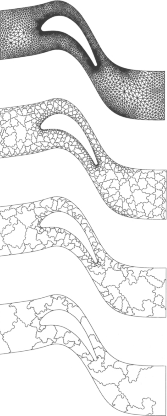
图9.9:二维聚合多重网格(中位对偶格式)生成粗网格。图序自上而下依次为最细网格与三个粗网格。
Problems of Agglomeration Multigrid 聚合多重网格的问题
对无黏流动,聚合多重网格的实现几乎没有困难。欧拉方程一般按各个控制体面上的通量来离散,因此控制体的形状多么复杂并不重要(实际上采用的是平均面向量)。此外,一阶精度的空间格式只需要相邻控制体内流动量的信息,而这些信息在粗网格上很容易获得。en
The implementation of agglomeration multigrid presents little difficulty for inviscid flows. The Euler equations are in general discretised as fluxes over individual control-volume faces. In this respect, it does not matter how complex is the shape of the control volume (in fact, averaged face vectors are used). Furthermore, a first-order accurate spatial scheme requires the knowledge of flow quantities in the neighbouring control volumes only. This information is readily available on the coarse grids.
对黏性流动,在任意形状的控制体上离散黏性通量不再那么直接,问题在于面中点处梯度的计算(参见文献[31]中的讨论)。另一个甚至更严重的困难与延拓算子所要求的精度有关。式(9.25)的不等式表明\(m_P = 2\),因为常用的限制算子(残差求和)只能给出\(m_R = 1\)。然而,在粗网格上构造线性插值并不容易。en
In the case of viscous flows, the discretisation of the diffusive fluxes on arbitrary shaped control volumes is no longer straightforward. The problem is the evaluation of gradients at face midpoints (see the discussion in [31]). Another, and even more serious, difficulty is related to the required accuracy of the prolongation operator. The inequality in Eq. (9.25) suggests \(m_P = 2\), since the common restriction operator (sum of residuals) leads to \(m_R = 1\) only. However, the construction of a linear interpolation is not easy on the coarse grids.
为了避免构造一阶精度的延拓算子,Mavriplis[53]提出采用常数延拓(即聚合粗网格体积内的所有细网格点都得到相同的解修正),并对黏性通量进行缩放。然而,这一做法无法达到最优的多重网格效率。en
In order to circumvent the construction of a first-order accurate prolongation operator, Mavriplis [53] proposed to use constant prolongation (i.e., all points of the fine grid contained within an agglomerated coarse-grid volume get the same solution correction) and a scaling of the viscous fluxes. However, this approach does not lead to optimal multigrid efficiency.
Haselbacher[31]建议在粗网格上也保留黏性通量的细网格离散,并像在最细网格上那样施加边界条件。此外,他提出了一种分段线性延拓算子。对标量量\(U\),它可以写成en
Haselbacher [31] suggested to retain the fine-grid discretisation of the viscous fluxes also on the coarse grids and to enforce the boundary conditions like on the finest grid. Moreover, he proposed a piecewise linear prolongation operator. For a scalar quantity \(U\), it can be written as
式(9.38)中的梯度\((\nabla\delta U_{2h})_i\)用5.3.4小节式(5.55)所述的线性最小二乘重构计算。限制器函数\(\Psi_i\)的值按5.3.5小节介绍的Barth-Jespersen限制器函数求值。en
The gradient \((\nabla\delta U_{2h})_i\) in Eq. (9.38) is calculated by using the linear least-squares reconstruction described in Subsection 5.3.4, Eq. (5.55). The values of the limiter function \(\Psi_i\) are evaluated according to the Barth-Jespersen limiter function presented in Subsection 5.3.5.