4.4 Discretisation of the Viscous Fluxes 黏性通量的离散化[cfd-4-4]

为了得到一致的空间离散ï¼黏性通量的控制体一般选取与对流通量相同。唯一的例外是采用重叠控制体的单元顶点格式(4.2.2小节)ï¼出于稳定性考虑[96]-[98]ï¼此时改用对偶控制体(4.2.3小节)。离散化控制方程(4.2)中的黏性通量 $\vec{F}_v$ ï¼与方程(4.17)、(4.22)、(4.37)、(4.42)类似ï¼由在控制体面上平均的变量计算。这与黏性通量的椭圆性质相符。因此ï¼计算黏性项(2.23)、(2.24)以及应力(2.15)所需的速度分量 $$(u, v, w)$$ 、动力黏度 $\mu$ 与热传导系数 $$k$$ 的值ï¼直接在面上取平均。在单元中心格式(图4.3与图4.8)情形ï¼控制体面 $$(I+1/2)$$ 处的值由下式给出en

The control volume for the viscous fluxes is generally chosen to be the same as for the convective fluxes in order to obtain a consistent spatial discretisation. An exception is made only in the case of the cell-vertex scheme with overlapping control volumes (Subsection 4.2.2), where the dual control volume (Subsection 4.2.3) is employed instead, primarily due to stability reasons [96]-[98]. The viscous fluxes $\vec{F}_v$ in the discretised governing equations (4.2) are, similar to Eqs. (4.17), (4.22), (4.37), (4.42), evaluated from variables averaged at the faces of the control volume. This is in line with the elliptic nature of the viscous fluxes. Thus, values of the velocity components $$(u, v, w)$$ , the dynamic viscosity $\mu$ , and of the heat conduction coefficient $$k$$ , which are required for the computation of the viscous terms (2.23), (2.24) and of the stresses (2.15), are simply averaged at a face. In the case of the cell-centred scheme (Figs. 4.3 and 4.8), the values at the face $$(I+1/2)$$ of the control volume result from

U_{I+1/2} = \frac{1}{2}(U_I + U_{I+1})\,, \tag{4.123}

其中 $$U$$ 为上述任一流动变量。两种单元顶点格式在面 $$(i+1/2)$$ 处同样如此——分别见图4.5与图4.8。en

where $$U$$ is any of the above flow variables. The same holds in the case of both cell-vertex schemes for the face $$(i+1/2)$$ - see Figs. 4.5 and 4.8, respectively.

剩下的任务是计算方程(2.15)中速度分量的一阶导数(梯度)与方程(2.24)中温度的一阶导数。这可以用以下两种方法之一完成:

有限差分;或
Green定理。

The remaining task is the evaluation of the first derivatives (gradients) of the velocity components in Eq. (2.15) and of the temperature in Eq. (2.24). This can be accomplished in one of two ways, i.e., by using

finite differences, or
Green's theorem.

第一种方法采用从笛卡尔坐标 $$(x, y, z)$$ 到曲线坐标 $(\xi, \eta, \zeta)$ 的局部变换ï¼例如en

The first approach applies a local transformation from Cartesian coordinates $$(x, y, z)$$ to the curvilinear coordinates $(\xi, \eta, \zeta)$ , e.g.,

\frac{\partial U}{\partial x} = \frac{\partial U}{\partial\xi}\frac{\partial\xi}{\partial x} + \frac{\partial U}{\partial\eta}\frac{\partial\eta}{\partial x} + \frac{\partial U}{\partial\zeta}\frac{\partial\zeta}{\partial x}\,, \text{ etc.} \tag{4.124}

导数 $U_\xi$ 、 $U_\eta$ 与 $U_\zeta$ 由有限差分近似得到ï¼更多细节见文献[96]-[98];坐标的导数与变换的Jacobian见附录A.1。本书更倾向于第二种方法ï¼它与本书讨论的有限体积方法学更为一致;不过ï¼它需要为导数的计算构造一个附加控制体。下面将针对单元中心格式与单元顶点格式分别讨论。一旦得到了控制体面上流动变量与一阶导数的值ï¼就可以按方程(4.2)把黏性通量的贡献累加起来;把这部分贡献加到无黏通量上ï¼空间离散即告完成ï¼随后便可对近似的控制方程进行时间积分。en

The derivatives $U_\xi$ , $U_\eta$ and $U_\zeta$ are obtained from finite difference approximations. More details can be found in Refs. [96]-[98]. See Appendix A.1 for the derivatives of the coordinates and for the Jacobian of the transformation. Here, we prefer the second approach, which is more in line with the finite volume methodology treated in this book. However, it requires the construction of an additional control volume for the computation of the derivatives. This will be discussed below for the cell-centred and the cell-vertex scheme. Once we obtained the values of the flow variables and of the first derivatives at the faces of the control volume, we can sum up the contributions due to the viscous fluxes according to Eq. (4.2). By adding the sum of the contributions to the inviscid fluxes, we completed the spatial discretisation, and we can thus integrate the approximated governing equations in time.

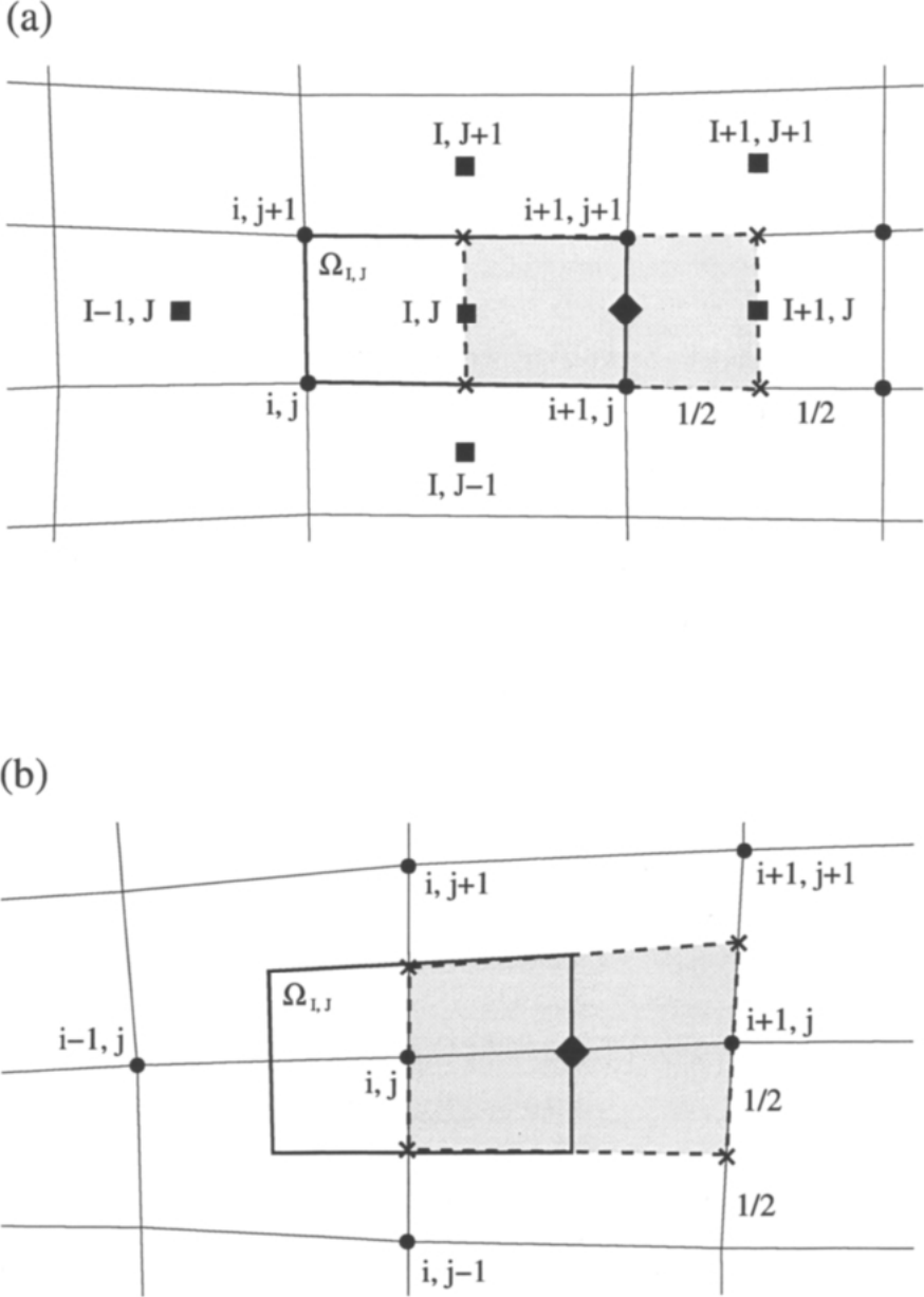
图4.12:用于计算一阶导数的辅助控制体Ω'(填充部分ï¼二维):(a)单元中心格式;(b)单元顶点格式

图4.12:用于计算一阶导数的辅助控制体 $\Omega'$ (填充部分ï¼二维):(a)单元中心格式;(b)单元顶点格式。图例:菱形符号标记一阶导数的计算位置;(a)中 $\Omega_{I,J}$ 为单元控制体ï¼单元中心以方块标记( $$I,J$$ 、 $$I+1,J$$ 、 $$I,J+1$$ 、 $$I+1,J+1$$ 等)ï¼网格点以圆点标记( $$i,j$$ 、 $$i+1,j$$ 、 $$i,j+1$$ 、 $$i+1,j+1$$ )ï¼面中点标记为 $$1/2$$ ;(b)中网格点为 $$i,j$$ 、 $$i-1,j$$ 、 $$i+1,j$$ 、 $$i,j+1$$ 、 $$i+1,j+1$$ 、 $$i,j-1$$ ï¼边中点以 $$1/2$$ 标记。

4.4.1 Cell-Centred Scheme 单元中心格式[cfd-4-4-1]

为了应用把一阶导数的体积分与 $$U$$ 的面积分联系起来的Green定理ï¼必须先定义一个合适的控制体。由于方程(4.2)中的求和需要面中点处的导数ï¼我们通过连接定义相邻网格单元的各边的中点ï¼构造一个以该面为中心的辅助控制体[31]、[19]、[98]ï¼如图4.12a所示。为了计算面 $$(I+1/2)$$ 处的一阶导数——在图4.12a中以菱形符号标记——必须把相应的流动变量 $$U$$ 沿辅助控制体的边界积分(以下以上标' 表示)。例如ï¼对x方向的导数en

In order to apply Green's theorem, which relates the volume integral of the first derivative to the surface integral of $$U$$ , we have to define a suitable control volume first. Since we need the derivatives at the midpoints of the faces for the summation in Eq. (4.2), we construct an auxiliary control volume centred at the face by connecting the midpoints of the edges defining adjacent grid cells [31], [19], [98] as shown in Fig. 4.12a. In order to evaluate the first derivative at the face $$(I+1/2)$$ - marked by a diamond symbol in Fig. 4.12a - we have to integrate the corresponding flow variable $$U$$ over the boundary of the auxiliary control volume (denoted by the superscript ' in the following). Thus, e.g., for the derivative in the x-direction

\frac{\partial U}{\partial x} = \frac{1}{\Omega'}\int_{\partial\Omega'} U\,dS'_x \approx \frac{1}{\Omega'}\sum_{m=1}^{N_F} U_m\,S'_{x,m}\,, \tag{4.125}

其中 $$N_F$$ 表示面的数目(二维 $$N_F = 4$$ ï¼三维 $$N_F = 6$$ )。体积 $\Omega'$ 与面向量 $\vec{S}'_m = [S'_{x,m}, S'_{y,m}, S'_{z,m}]^T$ 的分量按4.1节中已介绍的方法计算。面值 $$U_m$$ 或直接取单元中心值(即左、右面上的 $U_{i,j}$ 与 $U_{i+1,j}$ )ï¼或在上面与下面的面上取平均ï¼例如在 $$J+1/2$$ 处en

where $$N_F$$ stands for the number of faces ( $$N_F = 4$$ in 2D and $$N_F = 6$$ in 3D). The volume $\Omega'$ and the components of the face vector $\vec{S}'_m = [S'_{x,m}, S'_{y,m}, S'_{z,m}]^T$ , respectively, are computed as already presented in Section 4.1. The face values $$U_m$$ are obtained either directly as cell-centred values (i.e., $U_{i,j}$ and $U_{i+1,j}$ on the left and the right face), or by averaging like on the upper and the lower face, e.g., at $$J+1/2$$

U_{m_{I,J+1/2}} = \frac{1}{4}(U_{I,J} + U_{I+1,J} + U_{I,J+1} + U_{I+1,J+1})\,, \text{ etc.} \tag{4.126}

同样的方法可用于三维ï¼此时同样可用四个单元中心值作平均ï¼即en

We can apply the same approach in three dimensions, where again four cell-centred values can be utilised for the averaging. Hence,

\begin{aligned} U_{m_{I,J+1/2,K}} &= \frac{1}{4}(U_{I,J,K} + U_{I+1,J,K} + U_{I,J+1,K} + U_{I+1,J+1,K})\,,\\ U_{m_{I,J+1/2,K+1/2}} &= \frac{1}{4}(U_{I,J,K} + U_{I,J,K+1} + U_{I,J+1,K} + U_{I,J+1,K+1})\,, \end{aligned} \tag{4.127}

上述格式相当紧凑ï¼计算模板在二维只覆盖9个单元ï¼三维为15个。注意ï¼这种计算一阶导数的方法无法抑制两类虚假模态(相邻单元中心处解的失联)的产生[99]、[19]:一是棋盘格模态(chequer-board mode)ï¼源于围绕控制体的积分形式;二是一对波纹(搓衣板)模态ï¼源于相邻单元值的平均。不过ï¼实践中一般不会因此遇到困难。更严重的问题会出现在先把每个单元的梯度算出(类似对流通量的做法)、再在单元面上平均的做法中;这种做法看似更有吸引力ï¼但由于会导致强烈的奇偶失联ï¼并不推荐。en

The above scheme is quite compact, with the computational stencil extending over only nine cells in two dimensions and over 15 in three dimensions. It should be noted that this approach for computing the first derivatives cannot suppress the generation of two types of spurious modes (decoupled solutions at neighbouring cell centres) [99], [19]: the chequer-board mode, arising from the form of the integral around the control volume, and a pair of corrugated or washboard modes, arising from the averaging of values in neighbouring cells. However, there are generally no difficulties with this in practice. A more serious problem would occur, if the gradients would be first evaluated for each cell (similar to the convective fluxes) and then averaged at the cell faces. Although this approach may appear more attractive than the current methodology, it is not recommended since it leads to strong odd-even decoupling.

上述格式的缺点是:当网格不均匀时精度会下降[98]、[99]。就是说ï¼对任意拉伸的网格ï¼导数近似变得不相容(辅助控制体的形心不再对应面中心)。因此ï¼只有对适度且光滑拉伸的网格ï¼黏性通量才具有二阶精度的离散。最后ï¼应当指出,Navier-Stokes方程的TSL近似(2.4.3小节)很容易实现ï¼只需在计算梯度时略去相应的贡献即可。例如ï¼若边界层沿图4.12a的 $$I$$ 方向ï¼则辅助控制体左侧 $$(I, J)$$ 与右侧 $$(I+1, J)$$ 的贡献将被略去。en

A disadvantage of above scheme is a loss of accuracy if the grid is not uniform [98], [99]. Namely, for arbitrarily stretched grids the approximation of the derivatives becomes inconsistent (the centroid of the auxiliary control volume does no longer correspond to the face centre). Thus, the viscous fluxes are discretised with second-order accuracy only for moderately and smoothly stretched grids. Finally, it should be noted that the TSL approximation of the Navier-Stokes equations (Subsection 2.4.3) can easily be realised by omitting the appropriate contributions when computing the gradients. For example, if the boundary layer would be oriented along the $$I$$ -direction in Fig. 4.12a, contributions from the left $$(I, J)$$ and the right side $$(I+1, J)$$ of the auxiliary control volume would be dropped.

4.4.2 Cell-Vertex Scheme 单元顶点格式[cfd-4-4-2]

如前所述ï¼两种单元顶点格式的黏性通量离散都借助对偶控制体(4.2.3小节)。于是问题是如何在该控制体的面上计算一阶导数。考虑图4.12bï¼一种可能的做法是先在网格单元上积分求出单元中心处的梯度ï¼这在任意拉伸网格上具有一阶精度;下一步再像文献[31]、[100]那样ï¼把基于单元的梯度在控制体 $\Omega$ 的面上平均。然而ï¼这种做法无法防止解的奇偶失联。en

As already mentioned, both types of cell-vertex schemes resort to the dual control volume (Subsection 4.2.3) for the discretisation of the viscous fluxes. Hence, the question is how to evaluate the first derivatives at the faces of this control volume. Considering Fig. 4.12b, one possible alternative is to calculate the gradients at the cell centres first by integrating over the grid cells, which yields first-order accuracy on arbitrarily stretched grids. In a next step, the cell-based gradients are averaged at the faces of the control volume $\Omega$ like in Refs. [31], [100]. However, this approach cannot prevent an odd-even decoupling of the solution.

另一种与单元中心格式类似的做法ï¼是通过连接定义相邻网格单元的各边的中点ï¼围绕该面构造辅助控制体[101]、[102]ï¼如图4.12b所示。一阶差分的计算与单元中心格式的讨论相同ï¼必要时采用平均量。注意ï¼这一做法在形式上与有限差分近似完全相同[96]-[98]。该格式在任意拉伸网格上给出黏性通量的一阶精度离散ï¼在光滑网格上达到二阶精度[96]、[98]。另一个优点是计算模板很小:二维只有9个节点ï¼三维15个节点。en

Another possibility, similar to the cell-centred scheme, is to construct an auxiliary control volume around the face by connecting the midpoints of the edges defining adjacent grid cells [101], [102]. This is depicted in Fig. 4.12b. The evaluation of the first differences proceeds along the same lines as discussed for the cell-centred scheme, with averaged quantities where necessary. It should be noted that this approach is formally identical to the finite difference approximation [96]-[98]. This scheme leads to first-order accurate discretisation of the viscous fluxes on arbitrarily stretched grids and to second-order accuracy on smooth grids [96], [98]. Another positive feature is that the computational stencil is confined to only nine nodes in two dimensions and to 15 nodes in three dimensions.

最后ï¼还应提到另一种方法ï¼它选择了更复杂的积分路径ï¼平均时纳入所有相邻节点[20]。该格式的一个严重缺点是ï¼即使在二维也包含25点模板ï¼通常比紧凑模板引入更多数值扩散;此外ï¼若时间积分采用隐式格式ï¼通量Jacobian的带宽将变得过大而无法接受。关于梯度计算各种方法的详细讨论还可参见文献[103]。en

Finally, one further approach should be mentioned, where a more complex integration path was chosen, with averaging incorporating all neighbouring nodes [20]. A serious disadvantage of this scheme is that it encompasses a 25-point stencil even in two dimensions, which adds in general more numerical diffusion than compact stencils. Furthermore, if an implicit scheme would be envisioned for the time integration, the bandwidth of the flux Jacobian would become prohibitively large. A detailed discussion of various methodologies for the gradient evaluation can also be found in Ref. [103].