4.2.2 Cell-Vertex Scheme: Overlapping Control Volumes 单元顶点格式:重叠控制体[cfd-4-2-2]
在单元顶点格式中ï¼所有流动变量都与计算网格的节点相关联。在基于重叠控制体的做法中ï¼网格单元仍然充当控制体ï¼与单元中心格式的情形一样。区别在于:此时为各控制体算出的残差必须分配到网格点上[4]、[7]、[8]。图4.4示意了这一情形。en
In a cell-vertex scheme, all flow variables are associated with the nodes of the computational grid. Within the approach based on overlapping control volumes, the grid cells still represent the control volumes, just as in the case of the cell-centred scheme. The difference is that now the residuals computed for the control volumes have to be distributed to the grid points [4], [7], [8]. The situation is sketched in Fig. 4.4.
考察图4.4中的控制体\(\Omega_{I,J}\)ï¼它由下列节点定义en
Let us consider the control volume \(\Omega_{I,J}\) in Fig. 4.4, which is defined by the nodes
注意ï¼点\((i,j)\)位于\(\Omega_{I,J}\)的左下角。对流通量——例如对面\(\Delta S_{I,J-1/2}\)ï¼它由点\((i,j)\)与\((i+1,j)\)给定——近似为en
Note that the point \((i,j)\) is located at the lower left corner of \(\Omega_{I,J}\). The convective fluxes, e.g., for the face \(\Delta S_{I,J-1/2}\), which is given by the points \((i,j)\) and \((i+1,j)\), are approximated as
面中点处的变量用定义该面的两个节点上变量的算术平均来计算ï¼即en
The variables at the midpoint of the face are evaluated using an arithmetic average of the variables at the nodes defining the face, i.e.,
这一做法在三维中保持不变。例如ï¼对于与图4.1b中法向量\(\vec{n}_3\)相关联的面ï¼平均变量为en
The approach remains the same in three dimensions. For example, for the face associated with the normal vector \(\vec{n}_3\) in Fig. 4.1b, the averaged variables read
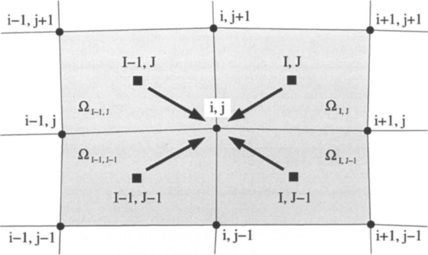
图4.4:单元顶点格式的重叠控制体(二维);箭头表示残差从单元形心向公共节点\(i,j\)的分配。图例:四个单元\(\Omega_{I-1,J-1}\)、\(\Omega_{I,J-1}\)、\(\Omega_{I-1,J}\)、\(\Omega_{I,J}\)(阴影四边形)共享公共节点\(i,j\)(实心圆点);各单元形心以实心方块标记\(I-1,J-1\)、\(I,J-1\)、\(I-1,J\)、\(I,J\);箭头表示把各单元(形心)的残差分配到公共节点;外圈网格点标记为\(i-1,j-1\)、\(i,j-1\)、\(i+1,j-1\)、\(i-1,j\)、\(i+1,j\)、\(i-1,j+1\)、\(i,j+1\)、\(i+1,j+1\)。
如果假定边1-2沿\(i\)方向、边1-5沿\(j\)方向、边1-4沿\(k\)方向ï¼并把点\((i,j,k)\)与图4.1b中的角点1相关联ï¼则方程(4.27)中的平均也可以写成en
If we assume the edge 1-2 being oriented in the \(i\)-direction, edge 1-5 in the \(j\)-direction, edge 1-4 in the \(k\)-direction, and if we finally associate the point \((i,j,k)\) with the corner 1 in Fig. 4.1b, the average in Eq. (4.27) can also be written as
对流通量于是同样由下式得到en
The convective flux is then again obtained from
把关系式(4.25)、(4.26)与(4.28)、(4.29)给出的所有面的贡献分别求和ï¼便得到所有网格单元的中间残差\(\vec{R}_{I,J,K}\)。为了把基于单元的残差与基于节点的残差联系起来ï¼还需要作进一步近似ï¼即采用残差分布公式(residual distribution formula)。它基本上是一个函数ï¼由共享该网格节点的所有单元的加权和来计算未知的基于节点的残差。已经提出的分布公式有:
- Ni的体积加权和[7];
- Hall的非加权求和[8];
- Rossow的特征(上风)加权方法[11]、[12]。
en
Summing up all face contributions given by relations (4.25), (4.26) and (4.28), (4.29), respectively, we obtain intermediate residuals \(\vec{R}_{I,J,K}\) for all grid cells. In order to relate the cell-based to the node-based residuals, a further approximation is made using a residual distribution formula. It is basically a function, which evaluates the unknown node-based residual from a weighted sum of all cells having the particular grid node in common. The following distribution formulae were devised:
- volume weighted sum due to Ni [7];
- non-weighted sum due to Hall [8];
- characteristic (upwind) weighting procedure of Rossow [11], [12].
对截断误差的理论研究[4]表明,Ni的格式比Hall的方法更精确。然而在实践中,Ni的分布公式在网格强烈扭曲和拉伸的地方会导致问题。例如ï¼使用O型网格时ï¼曾观察到翼型后缘附近压力场的强烈振荡[13]、[4]。此外ï¼只有把数值黏性加大很多才能获得收敛。上风加权方法[11]、[12]的基本思想与脉动分裂(fluctuation-splitting)格式[14]-[17]相当类似(参见3.1.5小节)ï¼但其数值实现要简单得多。从根本上说ï¼残差只沿特征方向向上游发送。en
Theoretical investigations of the truncation error [4] suggest that Ni's scheme is more accurate than Hall's approach. However, in practice Ni's distribution formula leads to problems in places, where the grid is strongly distorted and stretched. For example, strong oscillations of the pressure field near the trailing edge of an airfoil were observed when using O-grids [13], [4]. Furthermore, convergence could only be achieved when the numerical viscosity was increased considerably. The underlying idea of the upwind weighting procedure [11], [12] is quite similar to that of the fluctuation-splitting schemes [14]-[17] (cf. Subsection 3.1.5), but the implementation is numerically much simpler. Basically, the residuals are sent only upstream in the characteristic direction.
在这三种做法中,Hall的分布格式被证明最为稳健。在Hall的格式中ï¼某一节点处的残差由共享该节点的所有单元的中间残差\(\vec{R}_{I,J,K}\)直接求和得到。于是ï¼在图4.4所示的二维情形中ï¼我们得到en
Of the three approaches, Hall's distribution scheme proved to be the most robust. In Hall's scheme, the residual at a particular node results from a simple sum of all intermediate residuals \(\vec{R}_{I,J,K}\), which cells share the node. Thus, in the 2-D case rendered in Fig. 4.4, we get
在三维中ï¼必须以同样的方式把总共八个基于单元的残差求和。仔细考察(4.30)可以发现,\(\vec{R}_{i,j}\)恰好就是穿过超级单元(supercell)边界的净通量en
In three dimensions, in total eight cell-based residuals have to be summed up in the same way. A close inspection of (4.30) reveals that \(\vec{R}_{i,j}\) is just the net flux through the boundary of the supercell
这是因为穿过内部各面的通量互相抵消。超级单元也代表以点\((i,j)\)为中心的“总”控制体。在三维情形中ï¼总体积由以下单元构成en
due to the fact that the fluxes across the inner faces cancel each other. The supercell also represents the "total" control volume, centred at the point \((i,j)\). In the 3-D case, the total volume consists of the cells
从图4.4可以看出ï¼这些控制体至少重叠一个单元ï¼该格式正因此得名。en
As it can be seen from Fig. 4.4, the control volumes overlap by at least one cell, which gave the scheme its name.
源项用相应网格节点处的流动变量计算ï¼即en
The source term is calculated using the flow variables from the corresponding grid node, i.e.,