4.2.1 Cell-Centred Scheme 单元中心格式[cfd-4-2-1]

如果控制体与网格单元完全相同ï¼且流动变量位于网格单元的形心处(如图4.3所示)ï¼我们称之为单元中心格式(cell-centred scheme)。在计算离散化流动方程(4.2)时ï¼需要在单元的各个面上提供对流通量和黏性通量[6]。它们可以按以下三种方式之一来近似:

通量平均(average of fluxes)——由单元面左右两侧网格单元形心处的值分别计算通量ï¼再取平均ï¼但使用同一面向量(一般只用于对流通量);
变量平均(average of variables)——对与单元面左右两侧网格单元形心相关联的变量取平均;
由分别插值到单元面左右两侧的流动量计算通量(只用于对流通量)。

We speak of a cell-centred scheme if the control volumes are identical with the grid cells and if the flow variables are located at the centroids of the grid cells as indicated in Fig. 4.3. When we evaluate the discretised flow equations (4.2), we have to supply the convective and the viscous fluxes at the faces of a cell [6]. They can be approximated in one of the three following ways:

by the average of fluxes computed from values at the centroids of the grid cells to the left and to the right of the cell face, but using the same face vector (generally applied only to the convective fluxes);
by using an average of variables associated with the centroids of the grid cells to the left and to the right of the cell face;
by computing the fluxes from flow quantities interpolated separately to the left and to the right side of the cell face (employed only for the convective fluxes).

图4.3:单元中心格式的控制体(二维)

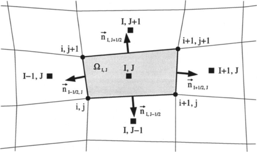
图4.3:单元中心格式的控制体(二维)。图例:阴影四边形 $\Omega_{I,J}$ 为控制体(即网格单元)ï¼其四个角点(实心圆点)为网格点 $$i,j$$ 、 $$i+1,j$$ 、 $$i,j+1$$ 、 $$i+1,j+1$$ ;实心方块 $$I-1,J$$ 、 $$I,J$$ 、 $$I+1,J$$ 、 $$I,J+1$$ 、 $$I,J-1$$ 表示各单元形心处流动变量的存储位置; $\vec{n}_{I+1/2,J}$ 、 $\vec{n}_{I-1/2,J}$ 、 $\vec{n}_{I,J+1/2}$ 、 $\vec{n}_{I,J-1/2}$ 为控制体各面的单位法向量。

以图4.3中的单元面 $\vec{n}_{I+1/2,J}$ 为例ï¼第一种做法——通量平均——在二维中写作en

Thus, taking the cell face $\vec{n}_{I+1/2,J}$ in Fig. 4.3 as an example, the first approach - average of fluxes - reads in two dimensions

\left(\vec{F}_c\,\Delta S\right)_{I+1/2,J} \approx \frac{1}{2}\left[\vec{F}_c(\vec{W}_{I,J}) + \vec{F}_c(\vec{W}_{I+1,J})\right]\Delta S_{I+1/2,J} \tag{4.15}

其中 $\Delta S_{I+1/2,J}$ 由方程(4.6)与(4.7)计算。en

with $\Delta S_{I+1/2,J}$ computed from Eqs. (4.6) and (4.7).

第二种可能的做法——变量平均——可以表述为en

The second possible approach - average of variables - can be formulated as follows

\left(\vec{F}\,\Delta S\right)_{I+1/2,J} \approx \vec{F}(\vec{W}_{I+1/2,J})\,\Delta S_{I+1/2,J}, \tag{4.16}

其中ï¼控制体面 $\vec{n}_{I+1/2,J}$ 上的守恒变量/因变量定义为两个相邻单元处数值的算术平均ï¼即en

where the conservative/dependent variables at the face $\vec{n}_{I+1/2,J}$ of the control volume are defined as the arithmetic average of values at the two adjacent cells, i.e.,

\vec{W}_{I+1/2,J} = \frac{1}{2}\left(\vec{W}_{I,J} + \vec{W}_{I+1,J}\right). \tag{4.17}

方程(4.16)中的通量向量 $\vec{F}$ 既可以指对流通量ï¼也可以指黏性通量。en

The flux vector $\vec{F}$ in Eq. (4.16) stands either for the convective or for the viscous fluxes.

第三种做法先把流动量(大多为速度分量、压力、密度和总焓)分别插值到单元面的两侧。插值得到的量——称为左(left)状态与右(right)状态(见4.3节开头)——在两侧一般并不相同。通过单元面的通量随后利用某个非线性函数由左、右状态之差求出。于是en

The third methodology starts with an interpolation of flow quantities (being mostly velocity components, pressure, density and total enthalpy) separately to both sides of the cell face. The interpolated quantities - termed the left and the right state (see the begin of Section 4.3) - differ in general between both sides. The fluxes through the cell face are then evaluated from the difference of the left and right state using some non-linear function. Hence,

\left(\vec{F}_c\,\Delta S\right)_{I+1/2,J} \approx f_{Flux}\left(\vec{U}_L,\,\vec{U}_R,\,\Delta S_{I+1/2,J}\right), \tag{4.18}

其中en

where

\begin{aligned} \vec{U}_L &= f_{Interp}\left(\cdots,\,\vec{U}_{I-1,J},\,\vec{U}_{I,J},\,\cdots\right) \\ \vec{U}_R &= f_{Interp}\left(\cdots,\,\vec{U}_{I,J},\,\vec{U}_{I+1,J},\,\cdots\right) \end{aligned} \tag{4.19}

它们表示插值得到的状态。当然ï¼与(4.15)–(4.19)类似的关系对其余单元面同样成立。en

represent the interpolated states. Of course, similar relations like (4.15)–(4.19) hold also for the other cell faces.

同样的近似也用于三维。例如ï¼在单元面 $\vec{n}_{I+1/2,J,K}$ (例如与图4.1b中的 $\vec{n}_2$ 相同)处ï¼方程(4.15)的通量平均变为en

The same approximations are employed in three dimensions. For example, at the cell face $\vec{n}_{I+1/2,J,K}$ (e.g., identical to $\vec{n}_2$ in Fig. 4.1b) the average of fluxes in Eq. (4.15) becomes

\left(\vec{F}_c\,\Delta S\right)_{I+1/2,J,K} \approx \frac{1}{2}\left[\vec{F}_c(\vec{W}_{I,J,K}) + \vec{F}_c(\vec{W}_{I+1,J,K})\right]\Delta S_{I+1/2,J,K} \tag{4.20}

其中 $\Delta S_{I+1/2,J,K}$ 按照与方程(4.8)和(4.9)相应的方式定义。变量平均则与方程(4.16)类似地写作en

with $\Delta S_{I+1/2,J,K}$ being defined correspondingly to Equations (4.8) and (4.9). The average of variables reads similarly to Eq. (4.16) as

\left(\vec{F}\,\Delta S\right)_{I+1/2,J,K} \approx \vec{F}(\vec{W}_{I+1/2,J,K})\,\Delta S_{I+1/2,J,K} \tag{4.21}

其中en

with

\vec{W}_{I+1/2,J,K} = \frac{1}{2}\left(\vec{W}_{I,J,K} + \vec{W}_{I+1,J,K}\right). \tag{4.22}

经由流动变量插值的做法ï¼则与方程(4.18)类似地给出en

The way over the interpolation of the flow variables results similarly to Eq. (4.18) in

\left(\vec{F}_c\,\Delta S\right)_{I+1/2,J,K} \approx f_{Flux}\left(\vec{U}_L,\,\vec{U}_R,\,\Delta S_{I+1/2,J,K}\right), \tag{4.23}

其中 $\vec{U}_L$ 与 $\vec{U}_R$ 是单元面上插值得到的数值。en

where $\vec{U}_L$ and $\vec{U}_R$ are the interpolated values at the cell face.

离散化流动方程(4.2)中尚待计算的最后一项是源项 $\vec{Q}$ 。如引言中所述ï¼源项通常假定在控制体内部为常数。因此ï¼它用相应单元中心处的流动变量来计算。于是ï¼我们可以定义en

The last term in the discretised flow equations (4.2) which remains to be evaluated is the source term $\vec{Q}$ . As we already stated in the introduction, the source term is usually supposed to be constant inside the control volume. For this reason, it is calculated using the flow variables from the corresponding cell centre. Hence, we may define

\left(\vec{Q}\,\Omega\right)_{I,J,K} = \vec{Q}(\vec{W}_{I,J,K})\,\Omega_{I,J,K}\,. \tag{4.24}

利用上述关系ï¼可以算出通过各面的通量ï¼并按照(4.2)完成对 $\Omega_{I,J,K}$ 边界的数值积分。换言之ï¼完整的残差 $\vec{R}_{I,J,K}$ 便得到了。在4.3节和4.4节中ï¼我们将进一步了解对流通量与黏性通量计算的细节。en

Using the above relations, the fluxes through the faces can be computed and the numerical integration over the boundary of $\Omega_{I,J,K}$ may be performed according to (4.2). In other words, the complete residual $\vec{R}_{I,J,K}$ is obtained. In Sections 4.3 and 4.4, we shall learn more about the details of the evaluation of the convective and viscous fluxes.