4.1.2 Three-Dimensional Case 三维情形[cfd-4-1-2]

与前述二维情形不同ï¼在三维中ï¼面向量与体积的计算存在一些困难。主要原因在于:一般情形下ï¼控制体一个面的四个顶点可能不共面。此时ï¼法向量在面上不再为常数(图4.2)。en

As opposed to the previous 2-D case, the calculation of face vectors and volumes poses some problems in three dimensions. The main reason for this is that, in general, the four vertices of the face of a control volume may not lie in a plane. Then, the normal vector is no longer constant on the face (Fig. 4.2). In

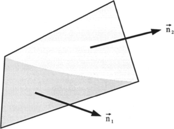
图4.2:三维中控制体一个面上法向量变化的情形

图4.2:三维中控制体一个面上法向量变化的情形。图例:阴影四边形为控制体的一个面;由于其四个顶点不共面ï¼面上的法向量(图中 $\vec{n}_1$ 、 $\vec{n}_2$ )随位置变化ï¼不再是常向量。

为了克服这一困难ï¼我们可以把控制体的全部六个面各自分解成两个或多个三角形ï¼而体积本身则由四面体拼成。以适当方式进行这种细分ï¼将得到一个在任意网格上至少一阶精度的离散格式[3]。当然ï¼数值代价会显著增加ï¼因为通量必须对每个部分三角形分别积分ï¼点操作次数至少加倍。然而ï¼文献[3]、[4]表明ï¼对于相当光滑、控制体面接近平行四边形的网格ï¼分解成三角形并不能明显提高解的精度。因此ï¼在下面的讨论中ï¼我们将对四边形面采用一种简化的处理方式ï¼它基于平均法向量(averaged normal vector)。en

order to overcome this difficulty, we could decompose all six faces of the control volume into two or more triangles each. The volume itself could then be built of tetrahedra. Performing this subdivision in an appropriate manner would lead to a discretisation scheme which is at least first-order accurate on arbitrary grids [3]. Of course, the numerical effort would be increased substantially, because the fluxes would have to be integrated over each partial triangle separately. Hence, the number of point operations would be at least doubled. However, in [3], [4] it is shown that for reasonably smooth grids, where the control volume faces approach parallelograms, the decomposition into triangles does not noticeably improve the solution accuracy. Therefore, we shall employ a simplified treatment of the quadrilateral faces in the following considerations, which is based on an averaged normal vector.

六面体控制体(如图4.1b所示)的面向量 $\vec{S}$ ï¼用与二维中计算四边形面积相同的Gauss公式来计算最为方便。例如ï¼对于面 $$m = 1$$ (图4.1b中的点1、5、8和4)ï¼先定义如下差分en

A face vector $\vec{S}$ of an hexahedral control volume, like that rendered in Fig. 4.1b, is most conveniently computed using the same Gauss's formula as employed in 2D for the area of a quadrilateral. Thus, e.g., for the face $$m = 1$$ (points 1, 5, 8 and 4 in Fig. 4.1b) we first define the differences

\begin{aligned} \Delta x_A &= x_8 - x_1, &\quad \Delta x_B &= x_5 - x_4, \\ \Delta y_A &= y_8 - y_1, &\quad \Delta y_B &= y_5 - y_4, \\ \Delta z_A &= z_8 - z_1, &\quad \Delta z_B &= z_5 - z_4. \end{aligned} \tag{4.8}

于是ï¼面向量 $\vec{S}_1 = \vec{n}_1\Delta S_1$ 由下式得出en

The face vector $\vec{S}_1 = \vec{n}_1\Delta S_1$ results then from

\vec{S}_1 = \frac{1}{2}\begin{bmatrix} \Delta z_A\,\Delta y_B - \Delta y_A\,\Delta z_B \\ \Delta x_A\,\Delta z_B - \Delta z_A\,\Delta x_B \\ \Delta y_A\,\Delta x_B - \Delta x_A\,\Delta y_B \end{bmatrix}. \tag{4.9}

其余五个面向量按类似方式计算。同样非常方便的做法是ï¼对每个控制体 $\Omega_{I,J,K}$ 只存储六个面向量中的三个(例如 $\vec{S}_1$ 、 $\vec{S}_3$ 与 $\vec{S}_5$ );其余面向量 $\vec{S}_2$ 、 $\vec{S}_4$ 与 $\vec{S}_6$ (经反号使其指向外侧)由相应的相邻控制体得到。方程(4.8)与(4.9)给出的是平均面向量。当面趋于平行四边形ï¼即面的全部顶点位于同一平面内时ï¼这一近似变为精确。单位法向量由方程(4.7)得到ï¼其中en

The five remaining face vectors are calculated in a similar manner. It is again very convenient to store only three of the six the face vectors (e.g., $\vec{S}_1$ , $\vec{S}_3$ , and $\vec{S}_5$ ) for each control volume $\Omega_{I,J,K}$ . The remaining face vectors $\vec{S}_2$ , $\vec{S}_4$ as well as $\vec{S}_6$ are obtained (with reversed signs to become outward facing) from the appropriate neighbouring control volumes. The above expressions in Eq. (4.8) and (4.9) deliver an average face vector. The approximation becomes exact when the face approaches a parallelogram, i.e., when the vertices of the face lie all in one plane. The unit normal vector is obtained from Eq. (4.7) with

\Delta S_m = \sqrt{S_{x,m}^2 + S_{y,m}^2 + S_{z,m}^2}\,. \tag{4.10}

计算一般六面体的体积有各种精度不一的公式(参见例如[1])。其中一种在多种应用中表现非常好的方法基于散度定理[5]。该定理把某一向量量的散度的体积分与其面积分联系起来。关键想法是取控制体 $\Omega$ 内某一点的空间位置——记作 $\vec{r} = [r_x, r_y, r_z]^T$ ——作为该向量量。据此ï¼散度定理写作en

Various, more or less accurate formulae are available for the calculation of the volume of a general hexahedron (see, e.g., [1]). One approach, which performed very well in various applications, is based on the divergence theorem [5]. This relates the volume integral of the divergence of some vector quantity to its surface integral. The key idea is to use the location in space of some point of the control volume $\Omega$ , let us call it $\vec{r} = [r_x, r_y, r_z]^T$ , as the vector quantity. Herewith, the divergence theorem reads

\int_{\Omega}\mathrm{div}(\vec{r})\,d\Omega = \oint_{\partial\Omega}\left(\vec{r}\cdot\vec{n}\right)dS\,. \tag{4.11}

方程(4.11)的左端很容易计算ï¼它给出的正是我们所要求的 $\Omega$ 的体积en

We can easily evaluate the left-hand side of Eq. (4.11) which gives us the volume of $\Omega$ that we are looking for

\int_{\Omega}\mathrm{div}(\vec{r})\,d\Omega = \int_{\Omega}\left(\frac{\partial r_x}{\partial x} + \frac{\partial r_y}{\partial y} + \frac{\partial r_z}{\partial z}\right)d\Omega = 3\,\Omega\,. \tag{4.12}

如果现在假定单位法向量在控制体的所有面上均为常数ï¼则方程(4.11)右端的面积分可以按如下方式求解en

If we assume now the unit normal vector is constant on all faces of the control volume, we can solve the surface integral on the right-hand side of Eq. (4.11) as follows

\oint_{\partial\Omega}\left(\vec{r}\cdot\vec{n}\right)dS \approx \sum_{m=1}^{m=6}\left(\vec{r}_{\mathrm{mid}}\cdot\vec{n}\right)_m\,\Delta S_m\,. \tag{4.13}

方程(4.13)中, $\vec{r}_{\mathrm{mid},m}$ 表示控制体第 $$m$$ 面的中点。例如en

In Eq. (4.13), $\vec{r}_{\mathrm{mid},m}$ denotes the midpoint of the control volume face $$m$$ . For example,

\vec{r}_{\mathrm{mid},1} = \frac{1}{4}\left(\vec{r}_1 + \vec{r}_5 + \vec{r}_8 + \vec{r}_4\right), \tag{7}

其中向量 $\vec{r}_1$ 、 $\vec{r}_5$ 、 $\vec{r}_8$ 与 $\vec{r}_4$ 对应图4.1b中面 $$m = 1$$ 的顶点1、5、8和4。其余各面的中点也有类似关系。方程(4.13)中面 $$m$$ 的面积 $\Delta S_m$ 由方程(4.10)得到。把方程(4.12)与(4.13)结合起来ï¼并用面向量 $\vec{S}$ 代替乘积 $\vec{n}_m\Delta S_m$ ï¼最终得到en

where the vectors $\vec{r}_1$ , $\vec{r}_5$ , $\vec{r}_8$ , and $\vec{r}_4$ correspond to the vertices 1, 5, 8, and 4 of the face $$m = 1$$ in Fig. 4.1b. Similar relations hold for the midpoints of the remaining faces. The area $\Delta S_m$ of the face $$m$$ in Eq. (4.13) is obtained from Eq. (4.10). Combining Equations (4.12) and (4.13) together, and inserting the face vector $\vec{S}$ for the product $\vec{n}_m\Delta S_m$ , we have finally the relationship

\Omega_{I,J,K} = \frac{1}{3}\sum_{m=1}^{m=6}\left(\vec{r}_{\mathrm{mid}}\cdot\vec{S}\right)_m \tag{4.14}

这就是控制体 $\Omega_{I,J,K}$ 体积的关系式。en

for the volume of the control volume $\Omega_{I,J,K}$ .

坐标系的原点原则上可以移到任何位置ï¼而不影响方程(4.14)的体积计算。这提示我们把原点放在控制体的某个顶点处(例如图4.1b中的点1)ï¼以获得更好的数值大小标度。于是ï¼我们可以把上述表达式(4.11)–(4.14)中的 $\vec{r}$ 替换为变换后的向量 $\vec{r}^{*}$ ï¼其定义为en

The origin of the coordinate system can be in principle moved to any place without affecting the volume calculation in Eq. (4.14). This leads us to the advice to locate the origin in one vertex of the control volume (e.g., point 1 in Fig. 4.1b), in order to achieve a better scaling of the numerical values. Thus, we may replace $\vec{r}$ in the above expressions (4.11)–(4.14) by a transformed vector $\vec{r}^{*}$ , which is defined as

\vec{r}^{*} = \vec{r} - \vec{r}_{\mathrm{origin}}\,. \tag{9}

需要特别指出ï¼用方程(4.14)算得的体积ï¼对于面为平面多边形的控制体是精确的。en

It is important to note that the volume computed with aid of Eq. (4.14) is exact for a control volume with planar faces.