3.2.1 Explicit Schemes 显式格式[cfd-3-2-1]
在方程(3.4)中令\(\beta=0\)、\(\omega=0\)ï¼便得到一个基本的显式时间积分格式。此时ï¼时间导数用前向差分近似ï¼残差只在当前时间层上计算(基于已知的流动量)ï¼即en
A basic explicit time-integration scheme is obtained by setting \(\beta=0\) and \(\omega=0\) in Eq. (3.4). In this case, the time derivative is approximated by a forward difference and the residual is evaluated at the current time level only (based on known flow quantities), i.e.,
其中质量矩阵已被集总。这是一个单步(single-stage)格式ï¼因为新解\(\vec{W}^{n+1}\)仅由一次残差计算得出。方程(3.7)没有实用价值ï¼因为它只有与一阶上风空间离散结合时才是稳定的。en
where the mass matrix was lumped. This represents a single-stage scheme, because a new solution \(\vec{W}^{n+1}\) results from only one evaluation of the residual. The scheme Eq. (3.7) is of no practical value, since it is stable only if combined with a first-order upwind spatial discretisation.
非常流行的是多步时间推进格式(Runge-Kutta 格式):解分若干步(stage)向前推进[64]ï¼残差在中间状态上计算ï¼并用系数对各步的残差加权。可以对这些系数进行优化ï¼以扩大稳定域、改善格式的阻尼特性ï¼从而提高其收敛性与稳健性[64]、[112]、[113]。而且ï¼依各步系数与步数而定ï¼多步格式还可以扩展到时间上的二阶或更高阶精度。人们还设计了特殊的 Runge-Kutta 格式ï¼在使允许时间步长最大化的同时ï¼保持 TVD 与 ENO 空间离散方法的性质[114]。en
Very popular are multistage time-stepping schemes (Runge-Kutta schemes), where the solution is advanced in several stages [64] and the residual is evaluated at intermediate states. Coefficients are used to weight the residual at each stage. The coefficients can be optimised in order to expand the stability region and to improve the damping properties of the scheme and hence its convergence and robustness [64], [112], [113]. Also, depending on the stage coefficients and the number of stages, a multistage scheme can be extended to 2nd- or higher-order accuracy in time. Special Runge-Kutta schemes were also designed to preserve the properties of the TVD and ENO spatial discretisation methods, while maximising the allowable time step [114].
显式多步时间推进格式可以与任何空间离散格式配合使用ï¼并且可以容易地在串行、向量以及并行计算机上实现。显式格式在数值上代价低廉ï¼所需计算机内存也很少。另一方面ï¼由于稳定性限制ï¼最大允许时间步长受到严格约束。对于黏性流动和高度拉伸的网格单元ï¼收敛到定常状态的过程会显著变慢。此外ï¼在方程组刚性很强(例如真实气体模拟、湍流模型)或源项刚性的情形下ï¼达到定常状态可能需要极长的时间;更糟的是ï¼显式格式可能变得不稳定ï¼或导致虚假的定常解[115]。en
Explicit multistage time-stepping schemes can be employed in connection with any spatial discretisation scheme. They can be easily implemented on serial, vector, as well as on parallel computers. Explicit schemes are numerically cheap, and they require only a small amount of computer memory. On the other hand, the maximum permissible time step is severely restricted because of stability limitations. Particularly for viscous flows and highly stretched grid cells, the convergence to steady state slows down considerably. Furthermore, in the case of stiff equation systems (e.g., real gas simulation, turbulence models), or of stiff source terms, it can take extremely long to achieve the steady state. Or even worse, an explicit scheme may become unstable or lead to spurious steady solutions [115].
如果我们只关心定常解ï¼便可以从若干种收敛加速方法学中选取(或组合使用)。第一种也是非常常用的技术是局部时间步进(local time-stepping):让每个控制体内的解以最大允许时间步长推进。这样ï¼向定常态的收敛会显著加快ï¼但瞬态解不再具有时间精度。另一种途径是所谓的特征时间步进(characteristic time-stepping):不仅使用逐点变化的时间步长ï¼而且每条方程(连续性、动量与能量方程)都用各自的时间步长积分。文献[116]针对二维 Euler 方程展示了这一概念的潜力。与特征时间步进类似的又一种加速技术是 Jacobi 预处理(Jacobi preconditioning)[117]-[119]。它基本上是一种点隐式 Jacobi 松弛ï¼在 Runge-Kutta 格式的每一步执行。可以把 Jacobi 预处理看作这样一种时间推进:所有波分量(通量雅可比矩阵的特征值)都被标度到相同的有效速度。它还在基本显式格式中加入了一个隐式分量。en
If we are interested in steady-state solutions only, we can select from (or combine) several convergence acceleration methodologies. The first, and very common, technique is local time-stepping. The idea is to advance the solution in each control volume with the maximum allowable time step. As a result, the convergence to the steady state is considerably accelerated. However, the transient solutions are no longer temporally accurate. Another approach is the so-called characteristic time-stepping. Here, not only locally varying time steps are used, but also each equation (continuity, momentum and energy equation) is integrated with its own time step. The potential of this concept was presented for 2-D Euler equations in Ref. [116]. A further acceleration technique, which is similar to the characteristic time-stepping is Jacobi preconditioning [117]-[119]. It is basically a point-implicit Jacobi relaxation, which is carried out at each stage of a Runge-Kutta scheme. Jacobi preconditioning can be seen as a time-stepping in which all wave components (eigenvalues of the flux Jacobian) are scaled to have the same effective speed. It also adds an implicit component to the basic explicit scheme.
另一种非常流行的加速方法ï¼是通过在显式格式中引入一定的隐式成分来增大最大可行时间步长ï¼称为隐式残差光滑(implicit residual smoothing)或残差平均(residual averaging)[120]、[121]。在结构网格上ï¼该方法要求对每个守恒变量求解一个三对角矩阵;在非结构网格上ï¼该矩阵通常用 Jacobi 迭代求逆。标准的隐式残差光滑允许把时间步长增大2至3倍。此外还发展了其他几种隐式残差光滑技术ï¼例如上风隐式残差光滑(upwind implicit residual smoothing)方法[122]ï¼它专为与上风空间离散配合使用而设计;与标准技术相比ï¼它允许显著更大的时间步长ï¼并改善了时间推进过程的稳健性[123]。还有一种方法是隐-显残差光滑(implicit-explicit residual smoothing)[124]、[125]ï¼用于改善时间离散在较大时间步长下的阻尼特性。en
Another very popular acceleration method is aimed at increasing the maximum possible time step by introducing a certain amount of implicitness in the explicit scheme. It is termed implicit residual smoothing or residual averaging [120], [121]. On a structured grid, the method requires the solution of a tridiagonal matrix for each conservative variable. In the case of unstructured grids, the matrix is usually inverted by means of Jacobi iteration. The standard implicit residual smoothing allows an increase of the time step by a factor of 2-3. Several other implicit residual smoothing techniques were developed. For example the upwind implicit residual smoothing methodology [122], which was designed to be employed together with an upwind spatial discretisation. In comparison to the standard technique, it allows for significantly larger time steps and it also improves the robustness of the time-stepping process [123]. One further method is the implicit-explicit residual smoothing [124], [125], which is intended to improve the damping properties of the time discretisation at larger time steps.
这里应当提到的最后一种、大概也是最重要的收敛加速技术是多重网格法(multigrid method)。它由 Fedorenko[126]与 Bakhvalov[127]于20世纪60年代在苏联发展ï¼用于求解椭圆型边值问题。这一方法学后来由 Brandt[128]、[129]进一步发展并推广。多重网格的思想基于这样的观察:迭代格式通常能非常有效地消除解中的高频误差(即控制体之间的振荡)ï¼但在消减低频(即全局)误差方面却表现相当差。因此ï¼在给定网格上推进解之后ï¼把它转移到较粗的网格上——在粗网格上ï¼低频误差部分地变成高频误差ï¼从而再次被迭代求解器有效阻尼。该过程在逐级变粗的一系列网格上递归重复ï¼每一层多重网格都有助于消灭一定频带宽度的误差。到达最粗网格后ï¼依次收集解的修正并插值回初始细网格ï¼在那里更新解。这一完整的多重网格循环不断重复ï¼直到解的变化小于给定阈值。为了进一步加速收敛ï¼还可以先在粗网格上启动多重网格过程ï¼执行若干个循环ï¼然后把解转移到较细的网格上再次执行多重网格循环;如此逐级重复ï¼直到最细网格。这一方法学称为完全多重网格(Full Multigrid,FMG)[129]。en
The last and probably the most important convergence acceleration technique, which should be mentioned here, is the multigrid method. It was developed in the 1960's in Russia by Fedorenko [126] and Bakhvalov [127]. They applied multigrid for the solution of elliptic boundary-value problems. The methodology was further advanced and promoted by Brandt [128], [129]. The idea of multigrid is based on the observation that iterative schemes usually eliminate high-frequency errors in the solution (i.e., oscillations between the control volumes) very effectively. On the other hand, they perform quite poor in reducing low-frequency (i.e., global) solution errors. Therefore, after advancing the solution on a given grid, it is transferred to a coarser grid, where the low-frequency errors become partly high-frequency ones and where they are again effectively damped by an iterative solver. The procedure is repeated recursively on a sequence of progressively coarser grids, where each multigrid level helps to annihilate a certain bandwidth of error frequencies. After the coarsest grid is reached, the solution corrections are successively collected and interpolated back to the initial fine grid, where the solution is then updated. This complete multigrid cycle is repeated until the solution changes less than a given threshold. In order to accelerate the convergence even further, it is possible to start the multigrid process on a coarse grid, carry out a number of cycles and then to transfer the solution to a finer grid, where the multigrid cycles are performed again. The procedure is then successively repeated until the finest grid is reached. This methodology is known as Full Multigrid (FMG) [129].
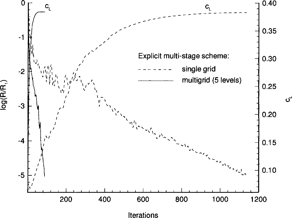
图3.7:NACA 0012翼型无黏跨声速流动的收敛历史;\(R\)——密度残差,\(c_L\)——升力系数。图例:图题栏"Explicit multi-stage scheme"(显式多步格式):虚线——single grid(单层网格);实线——multigrid (5 levels)(多重网格,5层)。横轴:Iterations(迭代次数);左纵轴:\(\log(R/R_0)\);右纵轴:\(c_L\)。
如前所述ï¼多重网格法最初是为求解椭圆型边值问题(Poisson 方程)而发展的ï¼在那里它非常高效。Jameson 首先提议把多重网格也用于 Euler 方程的求解[120]、[130]ï¼其途径基于所谓的完全近似存储(Full Approximation Storage,FAS)格式[129]ï¼即把多重网格直接应用于非线性控制方程。如今ï¼多重网格已成为求解 Navier-Stokes 方程的标准加速技术。结构网格上的实现例子见文献[131]-[136]ï¼非结构网格上的见文献[137]-[146]。虽然没有在椭圆型微分方程情形下那么快ï¼但已多次证明多重网格能把 Euler 或 Navier-Stokes 方程的求解加速5至10倍。跨声速流动的一个例子示于图3.7。近期研究还表明ï¼若把控制方程分解为双曲部分与椭圆部分ï¼可以实现更快的收敛[147]。我们将在9.4节再次回到多重网格方法学。en
As already mentioned, the multigrid method was originally developed for the solution of elliptic boundary-value problems (Poisson equation), where it is very efficient. Jameson first proposed to employ multigrid also for the solution of the Euler equations [120], [130]. The approach was based on the so-called Full Approximation Storage (FAS) scheme [129], where multigrid is directly applied to the non-linear governing equations. Nowadays, multigrid represents a standard acceleration technique for the solution of the Navier-Stokes equations. Examples of implementations can be found in Refs. [131]-[136] for structured grids, and in Refs. [137]-[146] for unstructured grids. Although not as fast as in the case of elliptic differential equations, it was often demonstrated that multigrid can accelerate the solution of the Euler or the Navier-Stokes equations by a factor between 5 and 10. An example for transonic flow is shown in Fig. 3.7. Recent research also revealed that faster convergence can be achieved if the governing equations are decomposed into hyperbolic and elliptic parts [147]. We shall return to the multigrid methodology again in Section 9.4.