3.1 Spatial Discretisation 空间离散[cfd-3-1]
让我们首先关注第一步——Navier-Stokes 方程的空间离散化ï¼也就是对流通量、黏性通量以及源项的数值近似。过去为此目的设计了许多不同的方法学ï¼而且发展仍在继续。为了对它们加以归类ï¼我们首先可以把空间离散格式分为如下三大类:有限差分、有限体积和有限元。所有这些方法都依赖某种网格来离散控制方程(2.19)。基本上存在两种不同类型的网格:
- 结构网格(structured grids)(图3.2)——每个网格点(顶点、节点)由索引\(i,j,k\)及相应的笛卡尔坐标\(x_{i,j,k}\)、\(y_{i,j,k}\)、\(z_{i,j,k}\)唯一标识。网格单元在二维为四边形ï¼在三维为六面体。如果网格像图3.1a那样是贴体的ï¼我们也称之为曲线网格(curvilinear grid)。
- 非结构网格(unstructured grids)(图3.3)——网格单元与网格点都没有特定的排列次序ï¼即相邻单元或相邻网格点无法由其索引直接确定(例如单元6与单元119相邻)。过去ï¼网格单元在二维为三角形ï¼在三维为四面体。如今ï¼为了恰当地分辨边界层ï¼非结构网格通常在二维由四边形与三角形的混合构成ï¼在三维由六面体、四面体、棱柱与四棱锥混合构成。因此ï¼这种情况我们称之为混合网格(hybrid 或 mixed grids)。
en
Let us at the beginning turn our attention to the first step - the spatial discretisation of the Navier-Stokes equations, i.e., the numerical approximation of the convective and viscous fluxes, as well as of the source term. Many different methodologies were devised for this purpose in the past and the development still continues. In order to sort them, we can at first divide the spatial discretisation schemes into the following three main categories: finite difference, finite volume, and finite element. All these methods rely on some kind of grid in order to discretise the governing equations (2.19). Basically, there exist two different types of grids:
- Structured grids (Fig. 3.2) - each grid point (vertex, node) is uniquely identified by the indices \(i,j,k\) and the corresponding Cartesian coordinates \(x_{i,j,k}\), \(y_{i,j,k}\), and \(z_{i,j,k}\). The grid cells are quadrilaterals in 2-D and hexahedra in 3-D. If the grid is body-fitted like in Fig. 3.1a, we speak also of curvilinear grid.
- Unstructured grids (Fig. 3.3) - grid cells as well as grid points have no particular ordering, i.e., neighbouring cells or grid points cannot be directly identified by their indices (e.g., cell 6 adjacent to cell 119). In the past, the grid cells were triangles in 2-D and tetrahedra in 3-D. Today, unstructured grids usually consist of a mix of quadrilaterals and triangles in 2-D and of hexahedra, tetrahedra, prisms and pyramids in 3-D, in order to resolve the boundary layers properly. Therefore, we speak in this case of hybrid or of mixed grids.
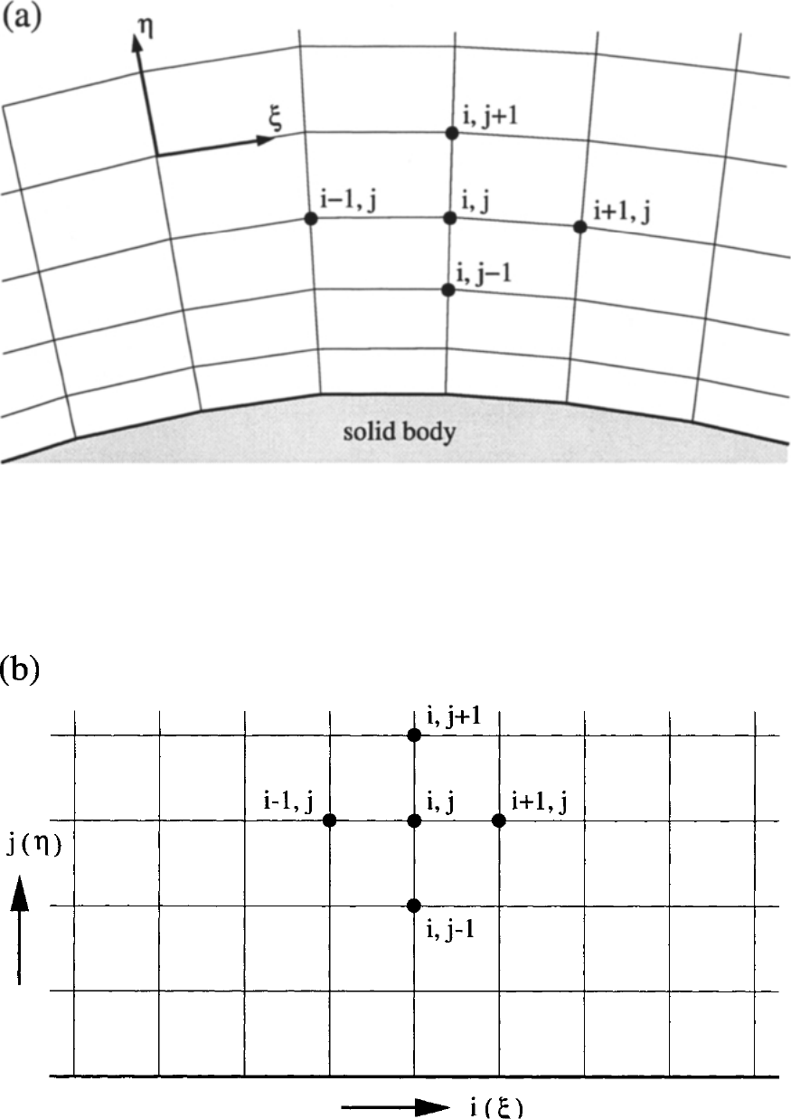
图3.2:结构化贴体网格方法(二维):(a)为物理空间;(b)为计算空间;\(\xi\)、\(\eta\)表示一个曲线坐标系。图例:(a)中\(\xi\)、\(\eta\)为沿网格方向的曲线坐标轴,solid body——固体壁面ï¼网格点标记为 i-1,j;i,j;i+1,j;i,j+1;i,j-1;(b)中坐标轴为 i(\(\xi\))与 j(\(\eta\))ï¼网格点标记同(a)。
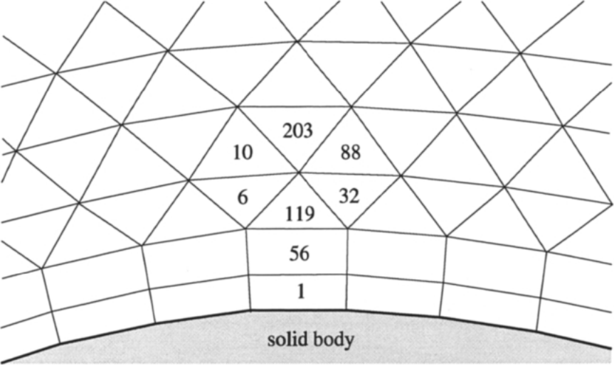
图3.3:二维非结构混合网格方法;数字标记各个单元。图例:solid body——固体壁面;图中数字(如1、56、119、6、32、88、10、203)为各单元编号ï¼近壁为四边形单元、外层为三角形与六边形单元的混合。
结构网格的主要优点源于这样一个性质:索引\(i,j,k\)构成一个线性地址空间——也称为计算空间(computational space)ï¼因为它直接对应于流动变量在计算机存储器中的存放方式。这一性质使得我们可以仅对相应的索引加减一个整数值ï¼就非常快捷、方便地访问某个网格点的邻居(例如(i+1)、(k-3)等——见图3.2)。可以想见ï¼梯度与通量的计算以及边界条件的处理都因这一特点而大为简化。隐式格式的实现也是如此ï¼因为通量雅可比矩阵排列规整、呈带状。但结构网格也有缺点ï¼那就是为复杂几何生成结构网格十分困难。如图3.4所示ï¼一种可能的做法是把物理空间划分成若干拓扑上更简单的部分——即块(blocks)——它们更容易被划分网格。因此我们称之为多块法(multiblock approach)[20]-[24]。当然ï¼流动求解器的复杂性随之增加ï¼因为需要专门的逻辑在各块之间交换物理量或通量。如果界面两侧的网格点可以彼此独立布置ï¼即允许网格线在块边界处不相互对接(如图3.4中C或F内部那样)ï¼灵活性还会进一步增加。那些只位于块界面一侧的网格点称为悬挂节点(hanging nodes)。这种做法的优点显而易见——网格线的数目可以按需要逐块单独选取。为这种增强的灵活性所付出的代价ï¼是悬挂节点守恒处理的开销增大[25]、[26]。多块方法学还为借助区域分解(domain decomposition)在并行计算机上实现流动求解器提供了有吸引力的可能性。然而ï¼对于复杂外形ï¼网格生成仍然需要很长的时间(往往数周或数月)。en
The main advantage of structured grids follows from the property that the indices \(i,j,k\) represent a linear address space - also called the computational space, since it directly corresponds to how the flow variables are stored in the computer memory. This property allows it to access the neighbours of a grid point very quickly and easily, just by adding or subtracting an integer value to or from the corresponding index (e.g., like (i+1), (k-3), etc. - see Fig. 3.2). As one can imagine, the evaluation of gradients, fluxes, and also the treatment of boundary conditions is greatly simplified by this feature. The same holds for the implementation of an implicit scheme, because of the well-ordered, banded flux Jacobian matrix. But there is also a disadvantage. This is the generation of structured grids for complex geometries. As sketched in Fig. 3.4, one possibility is to divide the physical space into a number of topologically simpler parts - blocks - which can be more easily meshed. We therefore speak of multiblock approach [20]-[24]. Of course, the complexity of the flow solver is increased, since special logic is required to exchange physical quantities or fluxes between the blocks. Additional flexibility is added, if the grid points at both sides of an interface can be placed independently of each other, i.e., if the grid lines are allowed not to meet at a block boundary (like inside C or F in Fig. 3.4). Those grid points, which are located only on one side of a block interface are called hanging nodes. The advantage of this approach is quite obvious - the number of grid lines can be chosen separately for each block as required. The price paid for the enhanced flexibility is an increased overhead for the conservative treatment of the hanging nodes [25], [26]. The multiblock methodology also offers interesting possibilities with respect to the implementation of the flow solver on a parallel computer by means of domain decomposition. However, very long times (often weeks or months) are still required for the grid generation in the case of complex configurations.
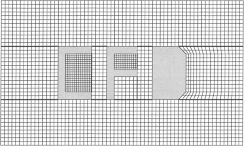
图3.4:具有相容/非相容块间界面的结构化多块网格;粗线表示块边界。图例:粗实线——块边界;字母C、F标示网格线在块边界处不相互对接(非相容界面)的区域。
另一种与块结构网格相关联的方法学是所谓的 Chimera 技术(嵌合网格技术)[27]-[32]。其基本思想是:先在计算域中每个几何体周围分别生成网格ï¼然后再把这些网格组合起来ï¼使它们在相遇处彼此重叠。图3.5以一个简单外形展示了这一情形。关键操作是在重叠区域于不同网格之间准确传递物理量。因此ï¼重叠范围要按照所需的插值阶数相应调整。与多块方法相比,Chimera 技术的优点是各片网格可以完全独立地生成ï¼而不必操心网格之间的界面。另一方面,Chimera 技术的问题在于:控制方程的守恒性质在重叠区域内得不到满足。en
Another methodology, related to block structured grids, represents the so-called Chimera technique [27]-[32]. The basic idea here is to generate first the grids separately around each geometrical entity in the domain. After that, the grids are combined together in such a way that they overlap each other where they meet. The situation is depicted in Fig. 3.5 for a simple configuration. The crucial operation is an accurate transfer of quantities between the different grids at the overlapping region. Therefore, the extension of the overlap is adjusted accordingly to the required interpolation order. The advantage of the Chimera technique over the multiblock approach is the possibility to generate the particular grids completely independent of each other, without having to take care of the interface between the grids. On the other hand, the problem of the Chimera technique is that the conservation properties of the governing equations are not satisfied through the overlapping region.
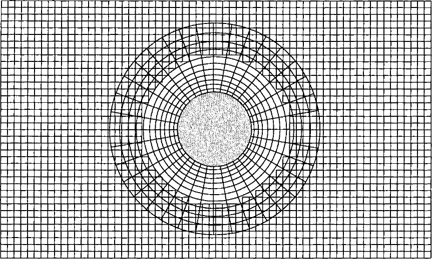
图3.5:Chimera技术示意(二维示例)。图例:背景为均匀笛卡尔网格ï¼物面附近为贴体的极坐标型网格ï¼两者相互重叠。
第二类网格是非结构网格。它们在处理复杂几何方面提供了最大的灵活性[33]。非结构网格的主要优点基于这样一个事实:三角形网格(二维)或四面体网格(三维)原则上可以自动生成ï¼而与计算域的复杂程度无关。当然ï¼实践中仍需适当设置一些参数才能获得高质量的网格。此外ï¼为了精确分辨边界层ï¼建议在固壁附近采用二维的矩形、三维的棱柱或六面体单元[34]-[41]。这类混合网格的另一个好处是减少了网格单元、棱边、面以及可能的网格点的数目。不过应当记住ï¼对于几何上要求苛刻的情形ï¼混合网格的生成并非易事。尽管如此ï¼为复杂外形生成非结构混合网格所需的时间仍显著低于多块结构网格所需的时间。由于流动模拟的几何保真度如今正在迅速提高ï¼快速、最少人机交互地生成网格的能力变得越来越重要ï¼在工业环境中尤其如此。非结构网格的又一优点是:与解相关的网格加密和粗化能够以相对自然、无缝的方式处理。谈及非结构方法的缺点ï¼其一是流动求解器内部必须采用复杂的数据结构。这类数据结构采用间接寻址ï¼依计算机硬件的不同ï¼会不同程度地降低计算效率。与结构格式相比ï¼内存需求一般也更高。尽管有种种困难ï¼在短时间内处理几何复杂问题的能力仍然重要得多。由此看来ï¼例如几乎所有商业 CFD 软件厂商都转而采用非结构流动求解器ï¼并不令人惊讶。关于非结构网格上空间与时间离散的各种方法学ï¼近期有一篇详细的综述见[42]。en
The second type of grids are the unstructured grids. They offer the largest flexibility in the treatment of complex geometries [33]. The main advantage of the unstructured grids is based on the fact that triangular (in 2-D) or tetrahedral grids (in 3-D) can be in principle generated automatically, independent of the complexity of the domain. In practice, it is of course still necessary to set some parameters appropriately, in order to obtain a good quality grid. Furthermore, in order to resolve the boundary layers accurately, it is advisable to employ in 2-D rectangular and in 3-D prismatic or hexahedral elements near solid walls [34]-[41]. Another benefit of such mixed grids is the reduction of the number of grid cells, edges, faces and possibly also of grid points. One should keep in mind though that the generation of mixed grids is not trivial for geometrically demanding cases. Nevertheless, the time required to built an unstructured, mixed grid for a complex configuration is still significantly lower than what is necessary for a multiblock structured grid. Since the geometrical fidelity of the flow simulations is nowadays rapidly increasing, the ability to generate grids fast and with minimum user interaction becomes more and more important. This is particularly true in industrial environment. Further advantage of unstructured grids is that solution dependent grid refinement and coarsening can be handled in a relatively native and seamless manner. To mention also the disadvantages of unstructured methods, one of them is the necessity to employ sophisticated data structures within the flow solver. Such data structures work with indirect addressing, which, depending on the computer hardware, leads to more or less reduced computational efficiency. The memory requirements are in general higher as compared to the structured schemes, too. But despite all difficulties, the capability to handle geometrically complex problems in short turn-around times still weights much more. From this point, it is not surprising that for example nearly all vendors of commercial CFD software switched over to unstructured flow solvers. A detailed review of various methodologies for spatial and temporal discretisation on unstructured grids appeared recently in [42].
网格生成之后ï¼下一个问题就是究竟如何离散控制方程。如前所述ï¼基本上可以在三种方法学之间选择:有限差分、有限体积和有限元。下面几小节将对它们逐一作简要讨论。en
Having generated the grid, the next question is how to actually discretise the governing equations. As we already said, we can basically choose between three methodologies: finite differences, finite volumes, and finite elements. We want to discuss all of them briefly in the next subsections.
3.1.1 Finite Difference Method 有限差分法[cfd-3-1-1]
有限差分法是最早应用于微分方程数值求解的方法之一ï¼由 Euler 于1768年(大概)首先使用。有限差分法直接应用于控制方程的微分形式。其原理是利用 Taylor 级数展开来离散流动变量的导数。为便于说明ï¼考察下面的例子。en
The finite difference method was among the first approaches applied to the numerical solution of differential equations. It was first utilised by Euler, probably in 1768. The finite difference method is directly applied to the differential form of the governing equations. The principle is to employ a Taylor series expansion for the discretisation of the derivatives of the flow variables. Let us for illustration consider the following example.
假设我们想计算某个标量函数\(U(x)\)在点\(x_0\)处的一阶导数。若把\(U(x_0+\Delta x)\)按\(x\)作 Taylor 级数展开ï¼便得到en
Suppose we would like to compute the first derivative of a scalar function \(U(x)\) at some point \(x_0\). If we develop now \(U(x_0+\Delta x)\) as a Taylor series in \(x\), we obtain
据此,\(U\)的一阶导数可近似为en
With this, the first derivative of \(U\) can be approximated as
上述近似是一阶的ï¼因为截断误差(记作\(\mathcal{O}(\Delta x)\))与余项中最大的项成正比ï¼并随\(\Delta x\)的一次方趋于零(关于精度的阶的讨论见第10章)。同样的步骤也可用来推导更精确的有限差分公式ï¼以及得到高阶导数的近似。en
The above approximation is of first order, since the truncation error (abbreviated as \(\mathcal{O}(\Delta x)\)), which is proportional to the largest term of the remainder, goes to zero with the first power of \(\Delta x\) (for a discussion on the order of accuracy see Chapter 10). The same procedure can be applied to derive more accurate finite difference formulae and to obtain approximations to higher-order derivatives.
有限差分方法学的一个重要优点是其简单性;另一个优点是容易获得高阶近似ï¼从而实现空间离散的高阶精度。另一方面ï¼由于该方法要求结构网格ï¼应用范围明显受限。此外ï¼有限差分法不能直接在贴体(曲线)坐标中使用ï¼而必须先把控制方程变换到笛卡尔坐标系——换言之ï¼从物理空间变换到计算空间(图3.2)。这里的问题在于坐标变换的雅可比行列式会出现在流动方程中(例如见附录A.1)。为避免引入额外的数值误差ï¼必须对该雅可比量进行一致地离散。因此ï¼有限差分法只能应用于相当简单的几何。如今ï¼它有时用于湍流的直接数值模拟(DNS)ï¼但很少用于工业应用。关于有限差分法的更多细节ï¼例如可参见[43]或有关偏微分方程求解的教科书。en
An important advantage of the finite difference methodology is its simplicity. Another advantage is the possibility to easily obtain high-order approximations, and hence to achieve high-order accuracy of the spatial discretisation. On the other hand, because the method requires a structured grid, the range of application is clearly restricted. Furthermore, the finite difference method cannot be directly applied in body-fitted (curvilinear) coordinates, but the governing equations have to be first transformed into a Cartesian coordinate system - or in other words - from the physical to the computational space (Fig. 3.2). The problem herewith is that the Jacobian of coordinate transformation appears in the flow equations (see, e.g., Appendix A.1). This Jacobian has to be consistently discretised in order to avoid the introduction of additional numerical errors. Thus, the finite difference method can be applied only to rather simple geometries. Nowadays, it is sometimes utilised for the direct numerical simulation of turbulence (DNS), but it is only very rarely used for industrial applications. More details to the finite difference method can be found for example in [43], or in textbooks on the solution of partial differential equations.
3.1.2 Finite Volume Method 有限体积法[cfd-3-1-2]
有限体积法直接利用守恒定律——即 Navier-Stokes/Euler 方程的积分形式。它由 McDonald[44]首先用于二维无黏流动的模拟。有限体积法离散控制方程的做法是:先把物理空间划分成若干任意多面体控制体ï¼然后用穿过控制体各个面的通量之和来近似式(2.19)右端的面积分。空间离散的精度取决于计算通量所用的具体格式。en
The finite volume method directly utilises the conservation laws - the integral formulation of the Navier-Stokes/Euler equations. It was first employed by McDonald [44] for the simulation of 2-D inviscid flows. The finite volume method discretises the governing equations by first dividing the physical space into a number of arbitrary polyhedral control volumes. The surface integral on the right-hand side of Equation (2.19) is then approximated by the sum of the fluxes crossing the individual faces of the control volume. The accuracy of the spatial discretisation depends on the particular scheme with which the fluxes are evaluated.
相对于网格ï¼控制体的形状与位置有几种不同的定义方式。可以区分出两种基本途径:
- 格心格式(cell-centred scheme)(图3.6a)——流动量存储在网格单元的形心处ï¼因此控制体与网格单元完全重合。
- 格点格式(cell-vertex scheme)(图3.6b)——流动变量存储在网格点上。此时控制体既可以取共享该网格点的所有单元的并集ï¼也可以取围绕该网格点居中的某个体积。前者称为重叠型控制体(overlapping control volumes)ï¼后者称为对偶控制体(dual control volumes)。
en
There are several possibilities of defining the shape and position of the control volume with respect to the grid. Two basic approaches can be distinguished:
- Cell-centred scheme (Fig. 3.6a) - here the flow quantities are stored at the centroids of the grid cells. Thus, the control volumes are identical to the grid cells.
- Cell-vertex scheme (Fig. 3.6b) - here the flow variables are stored at the grid points. The control volume can then either be the union of all cells sharing the grid point, or some volume centred around the grid point. In the former case we speak of overlapping control volumes, in the second case of dual control volumes.
我们将在后面两章讨论空间离散的内容时ï¼再详细比较格心与格点两种表述的优缺点。en
We shall discuss the advantages and disadvantages of cell-centred and cell-vertex formulations in both chapters on spatial discretisation.
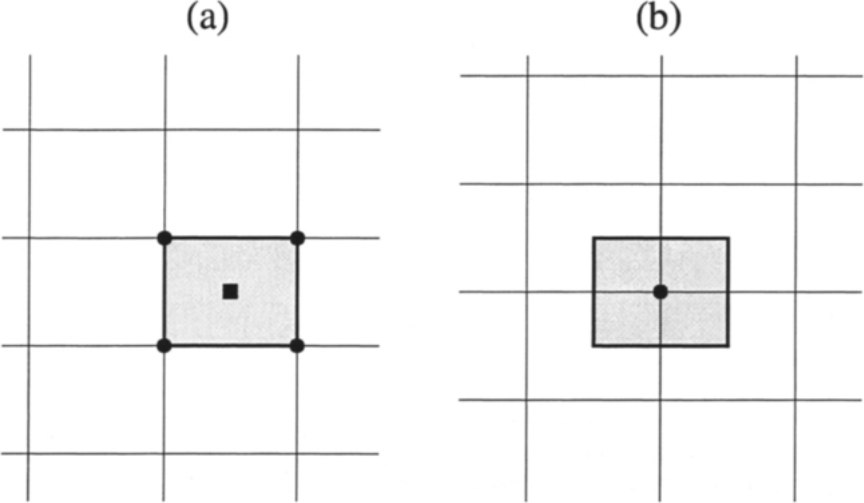
图3.6:格心格式(a)与格点格式(b)(对偶控制体)的控制体。图例:(a)中阴影四边形为控制体ï¼其四个角点(实心圆点)为网格点ï¼形心处的实心方块表示流动量的存储位置;(b)中阴影四边形为围绕中心网格点(实心圆点)的对偶控制体。
有限体积法的主要优点在于空间离散直接在物理空间中进行。因此ï¼不会像有限差分法那样遇到物理坐标系与计算坐标系之间的任何变换问题。与有限差分相比ï¼有限体积法的另一个优点是非常灵活——它既可以相当容易地在结构网格上实现ï¼也可以在非结构网格上实现。这使得有限体积法特别适合处理复杂几何中的流动。en
The main advantage of the finite volume method is that the spatial discretisation is carried out directly in the physical space. Thus, there are no problems with any transformation between the physical and the computational coordinate system, like in the case of the finite difference method. Compared to the finite differences, one further advantage of the finite volume method is that it is very flexible - it can be rather easily implemented on structured as well as on unstructured grids. This renders the finite volume method particularly suitable for the treatment of flows in complex geometries.
由于有限体积法基于对守恒定律的直接离散ï¼数值格式也使质量、动量和能量保持守恒。由此得到该方法的另一个重要特性ï¼即能够正确计算控制方程的弱解(weak solutions)。不过ï¼对于 Euler 方程还须满足一个附加条件ï¼即所谓的熵条件(entropy condition)。它之所以必要ï¼是因为弱解不唯一。熵条件可防止出现膨胀激波这类违反热力学第二定律(熵减小)的非物理现象。作为守恒离散的进一步结果ï¼跨越解的间断(如激波或接触间断)必须成立的 Rankine-Hugoniot 关系被直接满足。en
Since the finite volume method is based on the direct discretisation of the conservation laws, mass, momentum and energy are also conserved by the numerical scheme. This leads to another important feature of the method, namely the ability to compute weak solutions of the governing equations correctly. However, one additional condition has to be fulfilled in the case of the Euler equations. This is known as the entropy condition. It is necessary because of the non-uniqueness of the weak solutions. The entropy condition prevents the occurrence of unphysical features like expansion shocks, which violate the second law of thermodynamics (decrease of the entropy). As a further consequence of the conservative discretisation, the Rankine-Hugoniot relations, which must hold across a solution discontinuity (such as a shockwave or a contact discontinuity), are satisfied directly.
有趣的是ï¼在一定条件下可以证明有限体积法等价于有限差分法或低阶有限元法。凭借其吸引人的特性ï¼有限体积法如今广受欢迎、应用广泛。后续各章将对其进行介绍。en
It is interesting to note that under certain conditions, the finite volume method can be shown to be equivalent to the finite difference method, or to a low-order finite element method. Because of its attractive properties, the finite volume method is nowadays very popular and in wide use. It will be presented in the following chapters.
3.1.3 Finite Element Method 有限元法[cfd-3-1-3]
有限元法最初只用于结构分析ï¼由 Turner 等[45]于1956年首先提出。大约十年之后ï¼研究者们才开始把有限元法也用于连续介质中场方程的数值求解。然而ï¼直到20世纪90年代初ï¼有限元法才在 Euler 方程与 Navier-Stokes 方程的求解中流行起来。关于经典有限元方法学的一本很好的入门读物见[46];在流动问题中的应用见[47]、[48]ï¼以及更近期的[49]。en
The finite element method was originally employed for structural analysis only. It was first introduced by Turner et al. [45] in 1956. About ten years later, researchers started to use the finite element method also for the numerical solution of field equations in continuous media. However, only with the beginning of the 90's, did the finite element method gain popularity in the solution of the Euler and the Navier-Stokes equations. A good introduction into the classical finite element methodology can be found in [46]. Applications to flow problems are described in [47], [48], and more recently in [49].
有限元法应用于 Euler/Navier-Stokes 方程求解时ï¼一般从把物理空间细分为三角形单元(二维)或四面体单元(三维)开始ï¼因此需要生成非结构网格。根据单元类型和所需精度ï¼要在单元的边界上和/或内部指定一定数目的点ï¼流动问题的解要在这些点上求出。点的总数乘以未知量数目便确定自由度的数目。此外ï¼还须定义所谓的形函数(shape functions)ï¼它们表示解在一个单元内部的变化。实际实现中通常采用线性单元ï¼即只使用网格节点。此时形函数为线性分布ï¼在相应单元之外取值为零。这在光滑网格上给出二阶精度的解的表示。en
The finite element method, as it is in general applied to the solution of the Euler/Navier-Stokes equations, starts with a subdivision of the physical space into triangular (in 2-D) or into tetrahedral (in 3-D) elements. Thus, an unstructured grid has to be generated. Depending on the element type and the required accuracy, a certain number of points at the boundaries and/or inside an element is specified, where the solution of the flow problem has to be found. The total number of points multiplied with the number of unknowns determines the number of degrees of freedom. Furthermore, the so-called shape functions have to be defined, which represent the variation of the solution inside an element. In practical implementations, linear elements are usually employed, which use the grid nodes exclusively. The shape functions are then linear distributions, whose value is zero outside the corresponding element. This results in a second-order accurate representation of the solution on smooth grids.
在有限元法中ï¼需要把控制方程从微分形式变换为等价的积分形式。这可以通过两种不同的途径实现。第一种基于变分原理ï¼即寻找某个泛函取极值的物理解。第二种途径称为加权余量法(method of weighted residuals)或弱形式(weak formulation)ï¼它要求余量的加权平均值在整个物理域上恒等于零。余量可以看作解的近似误差。弱形式具有与守恒定律的有限体积离散相同的优点——可以处理激波等间断解。因此ï¼人们更倾向于采用弱形式而非变分方法。en
Within the finite element method, it is necessary to transform the governing equations from the differential into an equivalent integral form. This can be accomplished in two different ways. The first one is based on the variational principle, i.e., a physical solution is sought, for which a certain functional possesses an extremum. The second possibility is known as the method of weighted residuals or the weak formulation. Here, it is required that the weighted average of the residuals is identically zero over the physical domain. The residuals can be viewed as the errors of the approximation of the solution. The weak formulation has the same advantage as the finite volume discretisation of the conservation laws - it allows the treatment of discontinuous solutions such as shocks. Therefore, the weak formulation is preferred over the variational methodology.
有限元法的吸引人之处在于其积分形式与非结构网格的使用ï¼这两者对于复杂几何内部或周围的流动都更为有利。该方法还特别适合处理非牛顿流体。有限元法具有非常严格的数学基础ï¼对椭圆型和抛物型问题尤其如此。虽然在某些情形下可以证明该方法在数学上等价于有限体积离散ï¼但其数值工作量明显更高ï¼这也许可以解释为什么有限体积法变得更为流行。不过ï¼这两种方法有时会被结合使用——特别是在非结构网格上。例如ï¼边界处理和黏性通量的离散通常就是从有限元法那里"借"来的。en
The finite element method is attractive because of its integral formulation and the use of unstructured grids, which are both preferable for flows in or around complex geometries. The method is also particularly suitable for the treatment of non-Newtonian fluids. The finite element method has a very rigorous mathematical foundation, particularly for elliptic and parabolic problems. Although it can be shown in certain cases that the method is mathematically equivalent to the finite volume discretisation, the numerical effort is noticeably higher. This may explain why the finite volume method became more popular. However, both methods are sometimes combined - particularly on unstructured grids. So for example, the treatment of the boundaries and the discretisation of the viscous fluxes is usually "borrowed" from the finite element method.
3.1.4 Other Discretisation Methods 其他离散方法[cfd-3-1-4]
还有少数其他数值格式ï¼它们在实践中很少使用ï¼但在某些情形下却优于上面讨论的方法。这里简要提及两种具体途径。en
There are few other numerical schemes which are only seldom used in practice, but which are, in certain situations, superior to the methods discussed above. Two particular approaches should be mentioned here briefly.
Spectral Element Method 谱元法
第一个例子是谱元法(Spectral Element Method)[50]-[53]。谱元法把有限元技术的几何灵活性与谱格式的高阶空间精度(例如10阶)及快速收敛速率结合起来[54]。该方法基于解的高阶多项式表示(通常为 Lagrange 插值)ï¼并与标准 Galerkin 有限元法或加权余量法相结合。谱元法或者适用于高阶正则性有保证的特定问题ï¼或者适用于高阶正则性并不罕见的领域ï¼如不可压缩流体力学。它尤其适合涡流动。谱元法的优点主要在于其对流算子的无耗散、无频散近似ï¼以及对流-扩散边界层的良好近似。只要满足高阶正则性条件ï¼该方法就能处理几何与物理上都复杂的问题。除了适用范围相当狭窄之外ï¼谱元法的主要缺点是数值工作量非常高ï¼例如与有限体积法相比。en
The first such example is the Spectral Element Method [50]-[53]. The spectral element method combines the geometrical flexibility of the finite element technique with the high-order spatial accuracy (e.g., 10th-order) and the rapid convergence rate of the spectral schemes [54]. The method is based on a high-order polynomial representation of the solution (usually Lagrangian interpolants), combined with a standard Galerkin finite element method, or the method of weighted residuals. The spectral element method is appropriate either for a particular problem in which high-order regularity is guaranteed, or for which high-order regularity is not the exception, like in incompressible fluid mechanics. It is especially suitable for vortical flows. The advantage of the spectral element method is primarily its non-diffusive, non-dispersive approximation of the convection operator, and its good approximation of convection-diffusion boundary layers. The method can treat geometrically and physically complex problems, supposed the condition of high-order regularity is fulfilled. Apart from the rather narrow range of applications, the principal disadvantage of the spectral element method is its very high numerical effort as compared for example to the finite volume method.
Gridless Method 无网格方法
近来受到一定关注的另一种离散格式是所谓的无网格方法(Gridless Method)[55]-[57]。该方法只用点云进行空间离散ï¼不要求把点连接起来构成像传统结构或非结构网格格式那样的网格。无网格方法基于在笛卡尔坐标系中写出的控制方程微分形式ï¼利用围绕给定点的指定数目的邻居ï¼通过最小二乘重构来确定流动变量的梯度。无网格方法既不是有限差分、也不是有限体积或有限元途径ï¼因为它无须计算坐标变换、面积或体积。它可以视为有限差分法与有限元法的一种混合。无网格方法的主要优点是:求解复杂外形流动的灵活性(与非结构方法类似)ï¼以及在合适之处布点或聚点(或点云)的可能性。例如ï¼在计算梯度时可以轻而易举地只选取特征方向上的邻居。然而ï¼存在一个尚未解决的问题:虽然无网格方法求解的是 Euler 或 Navier-Stokes 方程的守恒律形式ï¼但质量、动量和能量的守恒是否真正得到保证并不清楚。en
Another discretisation scheme, which gained recently some interest, is the so-called Gridless Method [55]-[57]. This method employs only clouds of points for the spatial discretisation. It does not require that the points are connected to form a grid as in conventional structured or unstructured grid schemes. The gridless method is based on the differential form of the governing equations, written in the Cartesian coordinate system. Gradients of the flow variables are determined by a least-squares reconstruction, using a specified number of neighbours surrounding the particular point. The gridless method is neither a finite difference nor a finite volume or a finite element approach since coordinate transformations, face areas or volumes do not have to be computed. It can be viewed as a mix between the finite difference and the finite element method. The principal advantages of the gridless method are its flexibility in solving flows about complex configurations (similar to unstructured methods), and the possibility to locate or cluster the points (or the clouds of points) where it is appropriate. For example, it would be easily possible to select only the neighbours in the characteristic directions when computing gradients. However, there is one unresolved problem. Although the gridless method solves the conservation law form of the Euler or the Navier-Stokes equations, it is not clear whether conservation of mass, momentum and energy is really ensured.
无论选择哪种空间离散格式ï¼重要的问题是保证格式的一致性(consistency)ï¼即当网格充分加密时ï¼格式收敛于离散化方程的解。因此ï¼非常重要的是检查网格加密(例如把网格点数目加倍)后解改变了多少。如果解只有微小的改进ï¼我们称之为网格收敛解(grid converged solution)。另一个不言而喻的要求是:离散格式具有与所求解流动问题相称的精度阶。有时为了更快收敛ï¼这条规则会被放弃ï¼在工业环境中尤其如此(坏的解总比没有解好)。当然ï¼这是非常危险的做法。我们稍后将回到精度、稳定性与一致性的问题ï¼见第10章。en
Whichever spatial discretisation scheme we might select, it is important to ensure that the scheme is consistent, i.e., that it converges to the solution of the discretised equations, when the grid is sufficiently refined. It is therefore very important to check how much the solution changes, if the grid is refined (e.g., if we would double the number of grid points). If the solution improves only marginally, we speak of grid converged solution. Another rather self-evident requirement is that the discretisation scheme possesses the order of accuracy, which is appropriate for the flow problem being solved. This rule is sometimes given up in favour of faster convergence, particularly in industrial environment (bad solution is better than no solution). This is of course a very dangerous practice. We shall return to the question of accuracy, stability and consistency later in Chapter 10.
3.1.5 Central and Upwind Schemes 中心格式与上风格式[cfd-3-1-5]
到目前为止ï¼我们只讨论了空间离散可作的基本选择。但在上述三种主要方法——有限差分、有限体积和有限元——之中ï¼执行空间离散的数值格式多种多样。在此背景下ï¼把对流通量与黏性通量(分别为式(2.19)中的\(\vec{F}_c\)与\(\vec{F}_v\))的离散区分开来讨论会比较方便。鉴于黏性通量的物理性质ï¼唯一合理的方式是采用中心差分(中心平均)来离散它们ï¼因此它们在结构网格上的离散是直截了当的。在非结构的三角形或四面体网格上ï¼即便采用有限体积格式ï¼黏性通量也最好用 Galerkin 有限元方法学来近似[58]。对于非结构混合网格ï¼情形变得更为复杂ï¼此时对梯度作修正后的平均更为合适[59]-[63]。en
So far, we discussed only the basic choices which exist for the spatial discretisation. But within each of the above three main methods - finite difference, finite volume and finite element - various numerical schemes exist to perform the spatial discretisation. In this context, it is convenient to differentiate between the discretisation of the convective and the viscous fluxes (\(\vec{F}_c\) and \(\vec{F}_v\) in Eq. (2.19), respectively). Because of the physical nature of the viscous fluxes, the only reasonable way is to employ central differences (central averaging) for their discretisation. Thus, their discretisation on structured grids is straightforward. On unstructured triangular or tetrahedral grids, the viscous fluxes are best approximated using the Galerkin finite element methodology, even in the case of a finite volume scheme [58]. The situation becomes more complicated for unstructured mixed grids, where a modified averaging of gradients is more appropriate [59]-[63].
然而ï¼真正的多样性体现在对流通量的离散上。为了对各种方法学进行分类ï¼我们把注意力集中于为有限体积法发展的格式ï¼尽管其中多数概念同样可以直接应用于有限差分法或有限元法。en
However, the real variety is found in the discretisation of the convective fluxes. In order to classify the individual methodologies, we will restrict our attention to schemes developed for the finite volume method, although most of the concepts are also directly applicable to the finite difference or the finite element method.
Central Schemes 中心格式
第一类可以计入那些完全基于中心差分公式或中心平均的格式ï¼它们被称为中心格式(central schemes)。其原理是:为了计算控制体某个面上的通量ï¼把守恒变量向左、向右取平均。由于中心格式无法识别并抑制解的奇偶失联(odd-even decouplingï¼即产生离散化方程的两个相互独立的解)ï¼必须加入所谓的人工耗散(artificial dissipationï¼因其与黏性项相似而得名)以使其稳定。最广为人知的实现出自 Jameson 等[64]。在结构网格上ï¼它基于二阶差分与四阶差分的混合ï¼并以对流通量雅可比矩阵的最大特征值作为标度。在非结构网格上则采用未分割 Laplacian 算子与双调和算子的组合[65]。若对方程采用不同的标度因子ï¼该格式可以得到显著改进ï¼这一途径称为矩阵耗散格式(matrix dissipation scheme)[66]。应当指出ï¼在非结构混合单元网格上ï¼显式 Runge-Kutta 时间推进格式与常规中心格式结合时可能变得不稳定[67]。en
To the first category we may count schemes, which are based solely on central difference formulae or on central averaging, respectively. These are denoted as central schemes. The principle is to average the conservative variables to the left and to the right in order to evaluate the flux at a side of the control volume. Since the central schemes cannot recognise and suppress an odd-even decoupling of the solution (i.e., the generation of two independent solutions of the discretised equations), the so-called artificial dissipation (because of its similarity to the viscous terms) has to be added for stabilisation. The most widely known implementation is due to Jameson et al. [64]. On structured grids, it is based on a blend of 2nd- and 4th-differences scaled by the maximum eigenvalue of the convective flux Jacobian. A combination of an undivided Laplacian and biharmonic operator is employed on unstructured grids [65]. The scheme can be improved remarkably using different scaling factors for each equation. This approach is known as the matrix dissipation scheme [66]. It should be mentioned that on unstructured, mixed element grids the explicit Runge-Kutta time-stepping scheme can become unstable, when combined with the conventional central scheme [67].
Upwind Schemes 上风格式
另一方面ï¼还有更先进的空间离散格式ï¼它们是通过考虑 Euler 方程的物理性质而构造的。由于它们区分上游与下游的影响(波传播方向)ï¼故称为上风格式(upwind schemes)。这些格式大致可分为四大类:
- 通量向量分裂(flux-vector splitting);
- 通量差分分裂(flux-difference splitting);
- 总变差减小(total variation diminishing,TVD);以及
- 脉动分裂(fluctuation-splitting)格式。
下面各小节将对其中每一类作简要介绍。en
On the other hand, there are more advanced spatial discretisation schemes, which are constructed by considering the physical properties of the Euler equations. Because they distinguish between upstream and downstream influences (wave propagation directions), they are termed upwind schemes. They can be roughly divided into four main groups:
- flux-vector splitting,
- flux-difference splitting,
- total variation diminishing (TVD), and
- fluctuation-splitting schemes.
Each of these is described briefly in the following subsections.
Flux-Vector Splitting Schemes 通量向量分裂格式
其中一类的通量向量分裂格式ï¼依据某些特征变量的符号把对流通量向量分解为两部分ï¼这些特征变量一般与对流通量雅可比矩阵的特征值相似但不相同。通量向量的这两部分随后用偏上风的差分来离散。最早属于这种类型的通量向量分裂格式由 Steger 与 Warming[68]以及 Van Leer[69]于20世纪80年代初分别发展。第二类通量向量分裂格式则把通量向量分解为对流部分与压力(即声学)部分。Liou 等的 AUSM 格式(Advection Upstream Splitting Methodï¼迎风对流分裂方法)[70]、[71]ï¼以及 Jameson 的 CUSP 格式(Convective Upwind Split Pressureï¼对流上风分裂压力)[72]、[73]都利用了这一思想。进一步的类似途径还有 Edwards 提出的低耗散通量分裂格式(LDFSS,Low-Diffusion Flux-Splitting Scheme)[74]ï¼以及 Rossow 的基于马赫数的对流-压力分裂格式(MAPS,Mach number-based Advection Pressure Splitting)[75]、[76]。第二类通量向量分裂格式近来获得了更大的流行ï¼特别是因为它们改善了剪切层的分辨率ï¼而计算量只有中等水平。与通量差分分裂或 TVD 格式相比ï¼通量向量分裂格式的另一个优点是:它们可以相当容易地推广到真实气体流动。我们稍后再回到真实气体模拟。en
One class of the flux-vector splitting schemes decomposes the vector of the convective fluxes into two parts according to the sign of certain characteristic variables, which are in general similar to but not identical to the eigenvalues of the convective flux Jacobian. The two parts of the flux vector are then discretised by upwind biased differences. The very first flux-vector splitting schemes of this type were developed in the beginning of the 1980's by Steger and Warming [68] and by Van Leer [69], respectively. A second class of flux-vector splitting schemes decompose the flux vector into a convective and a pressure (an acoustic) part. This idea is utilised by schemes like AUSM (Advection Upstream Splitting Method) of Liou et al. [70], [71], or the CUSP scheme (Convective Upwind Split Pressure) of Jameson [72], [73], respectively. Further similar approaches are the Low-Diffusion Flux-Splitting Scheme (LDFSS) introduced by Edwards [74], or the Mach number-based Advection Pressure Splitting (MAPS) scheme of Rossow [75], [76]. The second group of flux-vector splitting schemes gained recently larger popularity particularly because of their improved resolution of shear layers, but only a moderate computational effort. An advantage of the flux-vector splitting schemes is also that they can be quite easily extended to real gas flows, as opposed to flux-difference splitting or TVD schemes. We shall return to real gas simulations further below.
Flux-Difference Splitting Schemes 通量差分分裂格式
第二类——通量差分分裂格式(flux-difference splitting schemes)——基于对界面上间断状态求解局部一维 Euler 方程ï¼这对应于 Riemann(激波管)问题。界面两侧的值通常称为左状态(left state)与右状态(right state)。在两个控制体之间的界面处求解 Riemann 问题的思想最早由 Godunov[77]于1959年提出。为了减少精确求解 Riemann 问题所需的数值工作量ï¼人们发展了近似 Riemann 求解器ï¼例如 Osher 等[78]与 Roe[79]的求解器。Roe 求解器至今仍经常使用ï¼因为它对边界层的分辨率极佳ï¼且对激波的表示十分清晰。它可以容易地在结构网格与非结构网格上实现[80]。en
The second group - flux-difference splitting schemes - is based on the solution of the locally one-dimensional Euler equations for discontinuous states at an interface. This corresponds to the Riemann (shock tube) problem. The values on either side of the interface are generally termed as the left and right state. The idea to solve the Riemann problem at the interface between two control volumes was first introduced by Godunov [77] back in 1959. In order to reduce the numerical effort required for an exact solution of the Riemann problem, approximate Riemann solvers were developed, e.g., by Osher et al. [78] and Roe [79]. Roe's solver is often used today because of its excellent resolution of boundary layers and a crisp representation of shocks. It can be easily implemented on structured as well as on unstructured grids [80].
TVD Schemes TVD 格式
TVD 格式的思想由 Harten[81]于1983年首先提出。TVD 格式基于一种旨在防止流动解中产生新极值的概念。TVD 格式的基本条件是:极大值必须不增ï¼极小值必须不减ï¼且不得产生新的局部极值。这样的格式称为保持单调性(monotonicity preserving)。因此ï¼具有 TVD 性质的离散方法学能够在没有任何虚假振荡的情况下分辨激波。TVD 格式一般实现为对流通量的平均再加上一个附加耗散项。该耗散项可以依赖也可以不依赖特征速度的符号。前一种情形称为上风 TVD 格式[82]ï¼后一种情形称为对称 TVD 格式[83]。经验表明应当优先选用上风 TVD 格式ï¼因为它对激波和边界层的分辨率优于对称 TVD 格式。TVD 格式的缺点是难以推广到高于二阶的空间精度。利用 ENO(Essentially Non-Oscillatoryï¼基本无振荡)离散格式[84]-[89]可以克服这一局限。en
The idea of TVD schemes was first introduced by Harten [81] in 1983. The TVD schemes are based on a concept aimed at preventing the generation of new extrema in the flow solution. The principal conditions for a TVD scheme are that maxima must be non-increasing, minima non-decreasing, and no new local extrema may be created. Such a scheme is called monotonicity preserving. Thus, a discretisation methodology with TVD properties allows it to resolve a shock wave without any spurious oscillations of the solution. The TVD schemes are in general implemented as an average of the convective fluxes combined with an additional dissipation term. The dissipation term can either depend on the sign of the characteristic speeds or not. In the first case, we speak of an upwind TVD scheme [82], in the second case of a symmetric TVD scheme [83]. The experience shows that the upwind TVD scheme should be preferred since it offers a better shock and boundary layer resolution than the symmetric TVD scheme. The disadvantage of the TVD schemes is that they cannot be easily extended to higher than second-order spatial accuracy. This limitation can be overcome using the ENO (Essentially Non-Oscillatory) discretisation schemes [84]-[89].
Fluctuation-Splitting Schemes 脉动分裂格式
最后一类——脉动分裂格式(fluctuation-splitting schemes)——提供了真正的多维上风。其目标是把那些与网格方向不一致的流动特征也精确分辨出来。与上面所有仅按网格单元方向对方程进行分裂的上风格式相比ï¼这是一个显著的优势。在脉动分裂方法学中ï¼流动变量与网格节点相关联;中间残差作为网格单元(二维为三角形ï¼三维为四面体)上的通量平衡来计算;然后把这些基于单元的残差以偏上风的方式分配到节点上;之后利用节点值更新解。对于方程组(Euler 或 Navier-Stokes 方程)ï¼基于单元的残差还须分解为标量波。由于这种分解在二维和三维都不唯一ï¼过去发展了若干种途径:从 Roe 的波模型[90]、[91]ï¼经 Sidilkover 的代数格式[92]ï¼直到最先进的特征分解方法[93]-[96]。尽管相对按维分裂的 Riemann、TVD 等求解器具有上述优势ï¼脉动分裂途径迄今仍只用于研究性代码ï¼其原因可归结为复杂性高、数值工作量大ï¼以及收敛问题。en
The last group - the fluctuation-splitting schemes - provides for true multidimensional upwinding. The aim is to resolve accurately also those flow features which are not aligned with the grid. This is a significant advantage over all above upwind schemes, which split the equations according only to the orientation of the grid cells. Within the fluctuation-splitting methodology, the flow variables are associated with the grid nodes. Intermediate residuals are computed as flux balances over the grid cells, which consists of triangles in 2-D and of tetrahedra in 3-D. The cell-based residuals are then distributed in an upwind-biased manner to the nodes. After that, the solution is updated using the nodal values. In the case of systems of equations (Euler or Navier-Stokes), the cell-based residuals have to be decomposed into scalar waves. Since the decomposition is not unique in 2-D and in 3-D, several approaches were developed in the past. The variety reaches from the wave model of Roe [90], [91] over the algebraic scheme of Sidilkover [92] to the most advanced characteristic decomposition method [93]-[96]. Despite the above mentioned advantage over the dimensionally split Riemann, TVD, etc. solvers, the fluctuation-splitting approaches are so far used only in research codes. This can be attributed to the complexity and the high numerical effort, as well as to convergence problems.
Central versus Upwind Schemes 中心格式与上风格式的比较
你也许会问:各种空间离散方法的收益与代价各是什么?一般而言ï¼与上风格式相比ï¼中心格式所需的数值工作量更低ï¼每次计算的 CPU 时间也更少。另一方面ï¼上风格式捕捉间断的精度远高于中心格式。此外ï¼由于其数值扩散较低ï¼上风格式可以用更少的网格点分辨边界层。特别是 Roe 的通量差分分裂格式与 CUSP 通量向量分裂格式能够非常精确地计算边界层。上风格式的负面效应在二阶或更高阶空间精度时显现:问题在于必须采用所谓的限制器函数(limiter functionsï¼或简称限制器 limiters)ï¼以防止在强间断附近产生虚假振荡。众所周知ï¼限制器会在光滑流动区域意外切换ï¼从而使迭代格式的收敛停滞。Venkatakrishnan[97]-[99]提出了一种补救措施ï¼对大多数实际问题效果令人满意ï¼但必须考虑到解中会出现微小波纹。限制器函数的另一个缺点是计算工作量大ï¼在非结构网格上尤其如此。en
You may ask now, what are the benefits and the drawbacks of the individual spatial discretisation methods. Generally speaking, central schemes require lower numerical effort, and hence less CPU time per evaluation, as compared to upwind schemes. On the other hand, upwind schemes are able to capture discontinuities much more accurately than central schemes. Furthermore, because of their lower numerical diffusion, the upwind schemes can resolve boundary layers using less grid points. Particularly, Roe's flux-difference splitting scheme and the CUSP flux-vector splitting scheme allow a very accurate computation of boundary layers. The negative side of the upwind schemes emerges for second- or higher-order spatial accuracy. The problem is that the so-called limiter functions (or simply limiters) have to be employed in order to prevent the generation of spurious oscillations near strong discontinuities. Limiters are known to stall the convergence of an iteration scheme, because of their accidental switching in smooth flow regions. A remedy was suggested by Venkatakrishnan [97]-[99], which works satisfactorily for most practical cases. However, small wiggles in the solution must be taken into account. Another disadvantage of the limiter functions is that they require high computational effort, particularly on unstructured grids.
Upwind Schemes for Real Gas Flows 真实气体流动的上风格式
针对真实气体模拟ï¼特别是化学反应流动ï¼已有若干对上风离散格式的推广。对于热力学与化学平衡的流体情形,Van Leer 通量向量分裂[69]与 Roe 近似 Riemann 求解器[79]的修改在文献[100]-[102]中给出。对于化学与热力学均处于非平衡的更复杂流动情形ï¼这两种上风方法的表述见[103]-[108]及其所引文献。其中文献[102]、[106]与[107]分别对上风离散格式所采用的方法学给出了很好的概述。最近ï¼文献[109]针对化学反应流动ï¼汇总了控制方程以及上风格式可能需要的雅可比矩阵和变换矩阵。en
With respect to real gas simulations, and in particular to chemically reacting flows, several extensions of the upwind discretisation schemes were presented. For the case of fluids in thermodynamic and chemical equilibrium, modifications of the Van Leer flux-vector splitting [69] and of Roe's approximate Riemann solver [79] were described in Refs. [100]-[102]. Formulations of the both upwind methods for the more complex case of flows with non-equilibrium chemistry and thermodynamics were provided in [103]-[108] and in the references cited therein. In particular, the articles [102], [106] and [107], respectively, give a good overview of the methodologies employed for the upwind discretisation schemes. Recently, a summary of the governing equations together with Jacobian and transformation matrices, which may be required by an upwind scheme, was presented in Ref. [109] for the case of chemically reacting flows.