9.5 Preconditioning for Low Mach Numbers 低马赫数预条件[cfd-9-5]
在低亚声速马赫数范围,当流动速度的大小与声速相比变得很小时,控制方程(2.19)的对流项呈现刚性。我们可以用下面的例子来演示这一点。在三维情形,我们有五个特征值en
In the low subsonic Mach number regime, when the magnitude of the flow velocity becomes small in comparison with the acoustic speed, the convective terms of the governing equations (2.19) become stiff. We can demonstrate this with the following example. In the 3-D case, we have the five eigenvalues
其中\(V\)表示逆变速度,\(c\)为声速。控制方程(按时间推进时)的刚性由特征条件数(condition number)决定。该数定义为最大特征值与最小特征值之比en
where \(V\) denotes the contravariant velocity and \(c\) the speed of sound. The stiffness of the governing equations (when marching in time) is determined by the characteristic condition number. This number is defined as the ratio of the largest to the smallest eigenvalue
允许的局部时间步长受最快的波限制,即受\((\Lambda_c)_4\)限制。在一个时间步内,最慢的波只移动了单元宽度的一小部分:\(\Lambda_{min}\Delta t \approx \left(\Lambda_{min}/\Lambda_{max}\right)h = h/C_N\)。因此,大的条件数\(C_N\)(即\(M \rightarrow 0\)时)会降低波传播的效率——它减慢向定常状态的收敛[78]。此外,文献[79]、[80]中证明,可压缩流动的格式所具有的人工耗散量在马赫数趋近于零时无法正确缩放。因此,这类空间离散在低马赫数下的精度会受损[81]。en
The allowable local time step is limited by the fastest wave, i.e, by \((\Lambda_c)_4\). During one time step, the slowest wave moves only over a fraction of the cell width: \(\Lambda_{min}\Delta t \approx \left(\Lambda_{min}/\Lambda_{max}\right)h = h/C_N\). Thus, a large condition number \(C_N\) (i.e., for \(M \rightarrow 0\)) reduces the efficiency of wave propagation - it slows down the convergence to steady state [78]. Furthermore, it was demonstrated in [79], [80] that schemes for compressible flows have an amount of artificial dissipation which does not scale correctly for Mach numbers approaching zero. Thus, the accuracy of such spatial discretisation suffers at low Mach numbers [81].
如果整个流场内的速度都很低(\(M < 0.2\)),那么压缩性效应可以忽略,并可以采用不可压缩方程。不可压缩Navier-Stokes方程可以用著名的压力基(pressure-based)格式求解[82]。另一种可能性是采用人工可压缩性(artificial compressibility,或称伪可压缩性)方法[83]-[89]。然而,存在如下类型的流动情形:
- 高速流动中内嵌大范围低速区域。一个例子是强收敛喷管上游的亚声速流动。
- 由于热源引起的密度变化而具有可压缩性的低速流动。表面传热或体积加热(燃烧模拟)时就会出现这种情况。
- 可压缩与不可压缩流动在不同马赫数下并存的问题——我们称之为全速流动(all-speed flows)。例如,在推进、高升力构型以及V/STOL机动中就会出现这种情形。
en
If the velocity in the entire flow field is low (\(M < 0.2\)), then the compressibility effects can be neglected and the incompressible equations can be utilised. The incompressible Navier-Stokes equations can be solved by the well-known pressure-based schemes [82]. The other possibility is the application of the artificial compressibility (or pseudo-compressibility) method [83]-[89]. However, there are flow cases like:
- high-speed flows with large embedded regions of low velocity. An example is the subsonic flow upstream of a strongly converging nozzle.
- Low-speed flows which are compressible due to density changes induced by heat sources. This occurs for surface heat transfer or volumetric heat addition (combustion simulation).
- Problems, where compressible and incompressible flow at varying Mach numbers occur side by side - we speak of all-speed flows. Such situation arises, for instance, in propulsion, for high-lift configurations and in V/STOL manoeuvring.
这些情形要求应用可压缩控制方程。为了在低马赫数下高效且精确地求解它们,可以采用预条件(preconditioning)。预条件的优点在于,它使得一种适用于所有马赫数的求解方法成为可能。下面,我们将推导预条件控制方程。en
Such cases require the application of the compressible governing equations. In order to solve them efficiently and accurately at low Mach numbers, preconditioning can be employed. The advantage of preconditioning is that it enables a solution method, which is applicable at all Mach numbers. In the following, we shall derive the preconditioned governing equations.
9.5.1 Derivation of Preconditioned Equations 预条件方程的推导[cfd-9-5-1]
我们以一维欧拉方程为例来演示预条件。它们可以写成微分形式en
We demonstrate preconditioning with the aid of 1-D Euler equations. They can be written in differential form as
其中\(\vec{W} = [\rho,\ \rho u,\ \rho E]^T\)为守恒变量向量,\(\vec{F}_c\)表示对流通量。为了考察预条件对谱半径(对时间步长的计算很重要)以及对流通量雅可比矩阵(对上风耗散很重要)的影响,把欧拉方程(9.41)改写为准线性形式en
where \(\vec{W} = [\rho,\ \rho u,\ \rho E]^T\) is the vector of conservative variables and \(\vec{F}_c\) denotes the convective fluxes. In order to see the effect of preconditioning on the spectral radii (important for the computation of the time step) and on the convective flux Jacobian (important for upwind dissipation), the Euler equations (9.41) are rewritten in the quasilinear form
其中\(\bar{A}_c = \partial\vec{F}_c/\partial\vec{W}\)为对流通量雅可比矩阵(参见附录A.2)。en
with \(\bar{A}_c = \partial\vec{F}_c/\partial\vec{W}\) being the convective flux Jacobian (cf. Appendix A.2).
低马赫数预条件背后的想法是变换控制方程(9.41),使新方程在低马赫数(即低于\(M \approx 0.2\))下具有更有利的性质。首先,我们希望均衡对流特征值,以约束条件数(见式(9.40)),从而消除\(M \rightarrow 0\)时的刚性。其次,我们希望改变数值耗散的缩放方式,以提高精度。最后,我们希望像压力基格式中那样把压力和速度耦合起来。这一变换用另一组流动变量取代守恒变量\(\vec{W}\)。可以有多种选择[90],但最常用的是压力、速度分量和温度。把式(9.42)中的准线性形式变换到新变量\(\vec{W}_p\),我们得到en
The idea behind low Mach-number preconditioning is to transform the governing equations (9.41) such that the new equations have more favourable properties at low Mach numbers (i.e. below \(M \approx 0.2\)). First of all, we want to equalise the convective eigenvalues in order to bound the condition number (see Eq. (9.40)) and thus to remove the stiffness at \(M \rightarrow 0\). We further want to change the scaling of the numerical dissipation in order to improve the accuracy. Finally, we want to couple the pressure and the velocity as it is done in the pressure-based schemes. The transformation replaces the conservative variables \(\vec{W}\) by a different set of flow variables. Various choices are possible [90], but the most often used are the pressure, the velocity components and the temperature. Transforming the quasilinear form in Eq. (9.42) into the new variables \(\vec{W}_p\), we obtain
在上面的式(9.43)中,\(\bar{P} = \partial\vec{W}/\partial\vec{W}_p\)表示从新变量\(\vec{W}_p\)到守恒变量\(\vec{W}\)的变换矩阵。引入新的通量雅可比矩阵en
In the above Eq. (9.43), \(\bar{P} = \partial\vec{W}/\partial\vec{W}_p\) represents the transformation matrix from the new variables \(\vec{W}_p\) into the conservative variables \(\vec{W}\). Introducing a new flux Jacobian
或等价地en
or equivalently
或者en
or
现在可以看到,守恒变量下的预条件方程(9.49)、(9.50)具有如下特点:
- 空间导数都乘以\(\bar{P}\bar{\Gamma}^{-1}\)。
- 非定常方程与式(9.42)的原始形式不同,因此解不再具有时间精度。
- 定常解(即\(\partial\vec{W}/\partial t = 0\))保持不变。
- 预条件系统的特征值和特征向量对应于矩阵\(\bar{P}\bar{\Gamma}^{-1}\bar{A}_c = \bar{P}\bar{\Gamma}^{-1}\bar{A}_{c,p}\bar{P}^{-1}\)的特征值和特征向量,因而与式(9.41)中原系统的不同。
en
We can see now that the preconditioned equations in the conservative variables (9.49), (9.50) have the following features:
- Spatial derivatives are multiplied by \(\bar{P}\bar{\Gamma}^{-1}\).
- Unsteady equations are different from the original form in Eq. (9.42) and hence the solution is no longer time accurate.
- Stationary solution (i.e. \(\partial\vec{W}/\partial t = 0\)) remains unchanged.
- Eigenvalues and eigenvectors of the preconditioned system correspond to those of the matrix \(\bar{P}\bar{\Gamma}^{-1}\bar{A}_c = \bar{P}\bar{\Gamma}^{-1}\bar{A}_{c,p}\bar{P}^{-1}\) and hence are different from those of the original system in Eq. (9.41).
现在的主要任务是找到一组合适的变量\(\vec{W}_p\)和矩阵\(\bar{\Gamma}\),使预条件系统(9.50)的对流特征值尽可能接近地被均衡。但同样重要的是,这些矩阵在\(M \rightarrow 0\)时必须仍有定义。此外,最好预条件系统在较高马赫数下能退化为原系统。en
The main task is now to find a suitable set of variables \(\vec{W}_p\) and the matrix \(\bar{\Gamma}\) such that the convective eigenvalues of the preconditioned system (9.50) are equalised as close as possible. But it is also important that the matrices remain defined for \(M \rightarrow 0\). Furthermore, it is desirable that the preconditioned system converts into the original system for higher Mach numbers.
在9.5.3小节给出变换矩阵和预条件矩阵之前,我们先讨论低马赫数预条件在流场解算器中的实现。en
Before we present the transformation and preconditioning matrices in Subsection 9.5.3, we shall discuss the implementation of the low Mach number preconditioning in a flow solver.
9.5.2 Implementation 实现[cfd-9-5-2]
采用显式多级格式(见6.1节所述)求解预条件控制方程(9.51)时,按以下步骤进行:
- 1. 基于矩阵\(\bar{P}\bar{\Gamma}^{-1}\bar{A}_c\)的谱半径计算新的时间步长。
- 2. 利用谱半径(如JST格式)或预条件通量雅可比矩阵的特征值和特征向量(如Roe上风格式)计算人工耗散。耗散项既可以在守恒变量下构造,也可以在原始变量下构造[90]。
- 3. 计算对流通量(或者不作改动,或者基于新变量\(\vec{W}_p\))。
- 4. 把耗散通量和对流通量相加。根据人工耗散的构造方式,或者将整个残差,或者仅将对流项乘以守恒变量预条件矩阵,即乘以\(\bar{P}\bar{\Gamma}^{-1}\)。
- 5. 将残差乘以\(\alpha_k\Delta t/V\)。
- 6. (可选)执行隐式残差光顺。
- 7. 从旧守恒变量\(\vec{W}^{(0)}\)中减去残差,以得到新守恒变量\(\vec{W}^{n+1}\)。
- 8. 更新边界条件(注意:所有基于特征变量的边界条件——如入流、出流、远场——都需要修改)。
en
The solution of the preconditioned governing equations (9.51) using an explicit multistage scheme (described in Section 6.1) proceeds according to the following steps:
- 1. Compute a new time step based on the spectral radii of the matrix \(\bar{P}\bar{\Gamma}^{-1}\bar{A}_c\).
- 2. Evaluate artificial dissipation using the spectral radii (e.g., JST scheme) or the eigenvalues and eigenvectors of the preconditioned flux Jacobian (e.g., Roe upwind scheme). The dissipation can be formulated either in the conservative or in the primitive variables [90].
- 3. Compute the convective fluxes (either without change or based on the new variables \(\vec{W}_p\)).
- 4. Sum up the dissipative and convective fluxes. Depending on the formulation of the artificial dissipation, either the whole residual or just the convective terms are multiplied by the conservative variable preconditioning matrix, i.e. by \(\bar{P}\bar{\Gamma}^{-1}\).
- 5. Multiply the residual by \(\alpha_k\Delta t/V\).
- 6. Carry out the implicit residual smoothing (optionally).
- 7. Subtract the residuals from the old conservative variables \(\vec{W}^{(0)}\) in oder to obtain the new conservative variables \(\vec{W}^{n+1}\).
- 8. Update the boundary conditions (note that all boundary conditions which are based on the characteristic variables - like inflow, outflow, farfield - need to be changed).
隐式格式遵循类似的步骤,只是省略第5步和第6步,并且守恒变量以不同的方式更新(参见6.2节)。还应注意,由于雅可比矩阵为\(\bar{P}\bar{\Gamma}^{-1}\bar{A}_c\),预条件必须包含在隐式算子中。en
Similar procedure is followed for an implicit scheme, only the steps 5. and 6. are omitted and the conservative variables are updated in a different way (cf. Section 6.2). It should also be noted that the preconditioning has to be included in the implicit operator since the Jacobian is \(\bar{P}\bar{\Gamma}^{-1}\bar{A}_c\).
预条件后的标量耗散格式(JST)取如下形式(见式(4.50))en
The preconditioned scalar dissipation scheme (JST) takes the form (see Eq. (4.50))
注意,如果之后要把整个残差乘以\(\bar{P}\bar{\Gamma}^{-1}\),就需要项\(\bar{\Gamma}\bar{P}^{-1}\),因为谱半径\(\hat{\Lambda}^S\)已经包含了预条件矩阵(因此它与式(4.53)不同)。在式(9.52)中,也可以把\(\bar{P}^{-1}\)与\(\vec{W}\)合并为\(W_p\)。这样,我们可以用原始变量表述预条件的标量耗散格式:en
Note that the term \(\bar{\Gamma}\bar{P}^{-1}\) is required if the complete residual is later multiplied by \(\bar{P}\bar{\Gamma}^{-1}\), since the spectral radius \(\hat{\Lambda}^S\) already contains the preconditioning matrix (thus it is different from Eq. (4.53)). It is also possible to combine \(\bar{P}^{-1}\) and \(\vec{W}\) into \(W_p\) in Eq. (9.52). Then, we can formulate the preconditioned scalar dissipation scheme in primitive variables as
必须认识到,此时只有对流通量乘以\(\Gamma^{-1}\),然后整个残差再乘以\(\bar{P}\)。式(9.53)的非守恒形式比关系式(9.52)稍微简单一些,但对于内流或含激波的流动存在精度问题。en
It is important to realize that in this case only the convective fluxes are multiplied by \(\Gamma^{-1}\) and the complete residual then by \(\bar{P}\). The nonconservative form in Eq. (9.53) is somewhat simpler than the relation (9.52), however there are problems with the accuracy for internal flows or for flows containing shocks.
预条件后的Roe上风格式可以写成(参见式(4.91))en
The preconditioned Roe upwind scheme can be written as (cf. Eq. (4.91))
其中\(|\bar{A}_{Roe}| = \bar{T}_{c,p}|\bar{\Lambda}_{c,p}|\bar{T}_{c,p}^{-1}\)。左特征向量(\(\bar{T}_{c,p}^{-1}\))、右特征向量(\(\bar{T}_{c,p}\))以及特征值(\(\bar{\Lambda}_{c,p}\))都是矩阵\(\bar{P}\bar{\Gamma}^{-1}\bar{A}_c = \bar{P}\bar{\Gamma}^{-1}\bar{A}_{c,p}\bar{P}^{-1}\)的。在\((I + 1/2)\)处的流动变量值由式(4.89)给出的Roe平均获得,并且整个残差乘以\(\bar{P}\bar{\Gamma}^{-1}\)。同样,式(9.54)的预条件Roe格式也可以用原始变量\(\vec{W}_p\)表述,这就得到en
where \(|\bar{A}_{Roe}| = \bar{T}_{c,p}|\bar{\Lambda}_{c,p}|\bar{T}_{c,p}^{-1}\). The left (\(\bar{T}_{c,p}^{-1}\)) and right (\(\bar{T}_{c,p}\)) eigenvectors, as well as the eigenvalues (\(\bar{\Lambda}_{c,p}\)) are those of the matrix \(\bar{P}\bar{\Gamma}^{-1}\bar{A}_c = \bar{P}\bar{\Gamma}^{-1}\bar{A}_{c,p}\bar{P}^{-1}\). Values of the flow variables at \((I + 1/2)\) are obtained by Roe's averaging given in Eq. (4.89), and the whole residual is multiplied by \(\bar{P}\bar{\Gamma}^{-1}\). Again, the preconditioned Roe scheme in Eq. (9.54) can be formulated in the primitive variables \(\vec{W}_p\) leading us to
此时,构成\(\bar{A}_{Roe,p}\)的特征值和特征向量由矩阵\(\Gamma^{-1}\bar{A}_{c,p}\)确定(参见式(9.47))。\(\Gamma^{-1}\bar{A}_{c,p}\)的特征值与\(\bar{P}\bar{\Gamma}^{-1}\bar{A}_c\)的特征值相同,即等于\(\bar{\Lambda}_{c,p}\),但特征向量不同。因此,式(9.55)中的Roe矩阵构成为\(|\bar{A}_{Roe,p}| = \bar{T}_p|\bar{\Lambda}_{c,p}|\bar{T}_p^{-1}\)。应当指出,在这种情形下,残差同样必须乘以\(\bar{P}\bar{\Gamma}^{-1}\),以便回到守恒变量。en
The eigenvalues and eigenvectors which compose \(\bar{A}_{Roe,p}\) are now determined by the matrix \(\Gamma^{-1}\bar{A}_{c,p}\) (cf. Eq. (9.47)). The eigenvalues of \(\Gamma^{-1}\bar{A}_{c,p}\) are identical to the eigenvalues of \(\bar{P}\bar{\Gamma}^{-1}\bar{A}_c\), i.e. to \(\bar{\Lambda}_{c,p}\), but the eigenvectors are different. Thus, the Roe matrix in Eq. (9.55) is composed as \(|\bar{A}_{Roe,p}| = \bar{T}_p|\bar{\Lambda}_{c,p}|\bar{T}_p^{-1}\). It should be mentioned that also in this case the residual has to be multiplied by \(\bar{P}\bar{\Gamma}^{-1}\) in order to obtain conservative variables.
9.5.3 Form of the Matrices 矩阵的形式[cfd-9-5-3]
在原始变量\(\vec{W}_p\)的各种选择中,形式en
Among the various choices for the primitive variables \(\vec{W}_p\), the form
出现得最多。因此,后面的讨论将局限于这一特定形式的\(\vec{W}_p\)。下面,我们将针对一般流体和完全气体,给出变换矩阵和预条件矩阵,以及特征值和左、右特征向量。en
appears most often. Therefore, we shall restrict the further discussion to this particular form of \(\vec{W}_p\). In the following, we will present the transformation and the preconditioning matrices together with the eigenvalues and the left and right eigenvectors for a general fluid, as well as a perfect gas.
Transformation matrices 变换矩阵
对于一般流体,从守恒变量到原始变量的变换矩阵\(\bar{P}^{-1} = \partial\vec{W}_p/\partial\vec{W}\)由文献[91]给出en
For a general fluid, the transformation matrix from the conservative into the primitive variables \(\bar{P}^{-1} = \partial\vec{W}_p/\partial\vec{W}\) is given by [91]
其中en
with
从原始变量到守恒变量的变换矩阵\(\bar{P} = \partial\vec{W}/\partial\vec{W}_p\)为[91]en
The transformation matrix from the primitive into the conservative variables \(\bar{P} = \partial\vec{W}/\partial\vec{W}_p\) reads [91]
其中\(\alpha_p\)和\(\alpha_T\)分别为定压和定温压缩性系数。声速可以由下式计算en
where \(\alpha_p\) and \(\alpha_T\) are the compressibility coefficients at constant pressure and temperature, respectively. The speed of sound can be computed from
对于完全气体(见2.4.1小节),式(9.60)中的压缩性系数成为\(\alpha_p = 1/p\)和\(\alpha_T = 1/T\)。此时,式(9.57)中从守恒变量到原始变量的变换矩阵\(\bar{P}^{-1} = \partial\vec{W}_p/\partial\vec{W}\)可以写成en
In the case of a perfect gas (see Subsection 2.4.1), the compressibility coefficients in Eq. (9.60) become \(\alpha_p = 1/p\) and \(\alpha_T = 1/T\). In this case, the transformation matrix from the conservative into the primitive variables \(\bar{P}^{-1} = \partial\vec{W}_p/\partial\vec{W}\) from Eq. (9.57) can be cast into
对完全气体,从原始变量到守恒变量的变换矩阵\(\bar{P} = \partial\vec{W}/\partial\vec{W}_p\)为en
The transformation matrix from the primitive into the conservative variables \(\bar{P} = \partial\vec{W}/\partial\vec{W}_p\) reads for a perfect gas
Preconditioning matrices 预条件矩阵
在欧拉方程的情形下,预条件矩阵的构造相对容易。van Leer等人[92]提出的构造达到了可达的最低条件数。该方法在文献[79]中有详细讨论。然而,Navier-Stokes方程的预条件则更为复杂,原因在于黏性项会导致复数波速,使预条件系统难以分析。黏性流动最著名的预条件器分别由Choi和Merkle[93]、[94],Turkel[90]、[95]-[97],Lee和van Leer[98]、[99]以及Lee[80],Jorgenson和Pletcher[100],以及Weiss和Smith[101]、[45]提出。应用实例见文献[91]、[102]-[109]。en
The construction of a preconditioning matrix is relatively easy in the case of the Euler equations. The formulation proposed by van Leer at al. [92] achieves the lowest attainable condition number. The methodology was discussed in detail in [79]. However, the preconditioning of the Navier-Stokes equations is more involved. The reason is that the viscous terms lead to complex wave speeds, which makes the preconditioned system difficult to analyse. The most recognised preconditioners for viscous flows were proposed by Choi and Merkle [93], [94], Turkel [90], [95]-[97], Lee and van Leer [98], [99] and Lee [80], Jorgenson and Pletcher [100], and by Weiss and Smith [101], [45], respectively. Examples of applications can be found in Refs. [91], [102]-[109].
Weiss and Smith Preconditioner Weiss和Smith预条件器
Weiss和Smith[101]、[45]提出的预条件矩阵\(\bar{\Gamma}\),在一般流体情形下,其形式与式(9.59)中的\(\bar{P}\)相同,只是把\(\rho_p\)替换为适当的预条件参数(preconditioning parameter)\(\theta\)。预条件矩阵的逆也是如此,即\(\bar{\Gamma}^{-1}\)与式(9.57)中的\(\bar{P}^{-1}\)类似。因此,式(9.58)中的参数\(a_1\)变为en
The preconditioning matrix \(\bar{\Gamma}\) due to Weiss and Smith [101], [45] has, in the case of a general fluid, a form identical to \(\bar{P}\) in Eq. (9.59) with \(\rho_p\) replaced by a suitable preconditioning parameter \(\theta\). The same holds also for the inverse of the preconditioning matrix, i.e., \(\bar{\Gamma}^{-1}\) which resembles \(\bar{P}^{-1}\) from Eq. (9.57). Consequently, the parameter \(a_1\) from Eq. (9.58) is changed into
对于完全气体,预条件矩阵\(\bar{\Gamma}\)可以写成en
In the case of a perfect gas, the preconditioning matrix \(\bar{\Gamma}\) can be written as
其中\(\theta\)仍是预条件参数,稍后定义。预条件矩阵的逆由下式给出en
where \(\theta\) is again the preconditioning parameter, which will be defined later. The inverse of the preconditioning matrix is given by
其中采用缩写en
with the abbreviations
相应地,对完全气体,en
or, correspondingly for a perfect gas,
其中\(\Delta h\)是控制体尺寸的度量,\(\Delta p\)表示相邻控制体之间的压差,\(\epsilon\)是一个小数(\(\approx 10^{-3}\))。从式(9.70)的定义可以看到,参考速度受局部输运速度的限制。\(\nu/\Delta h\)和\(\kappa/\Delta h\)两项在以扩散或热传导为主的边界层内变得重要。压力项的目的是防止\(u_r\)在驻点处趋于零。当\(u_r = c\)时,\(\bar{\Gamma}\)变得与\(\bar{P}\)完全相同,\(\bar{\Gamma}^{-1}\)则变为\(\bar{P}^{-1}\)。因此,正如所期望的那样,预条件在超声速流动时自动关闭。en
where \(\Delta h\) is a measure of the control volume size, the quantity \(\Delta p\) stands for the pressure difference between the adjacent control volumes and \(\epsilon\) is a small number (\(\approx 10^{-3}\)). As we can see from the definition in Eq. (9.70), the reference velocity is bounded by the local transport velocity. The terms \(\nu/\Delta h\) and \(\kappa/\Delta h\) become important in boundary layers with dominant diffusion or heat conduction. The pressure term is intended to prevent \(u_r\) from vanishing at stagnation points. In the case that \(u_r = c\), \(\bar{\Gamma}\) becomes identical to \(\bar{P}\) and \(\bar{\Gamma}^{-1}\) is converted into \(\bar{P}^{-1}\). Hence, the preconditioning is turned off for a supersonic flow as intended.
另一种针对完全气体的做法是令[104]en
Another possibility, which was devised for a perfect gas, is to set [104]
其中参考马赫数由下式给出en
with the reference Mach number given by
而\(M\)为当地马赫数(\(M^2 = \|\vec{v}\|_2^2/c^2\))。按照文献[104],参数\(M^2_{min} = K M_\infty^2\)且\(K \approx 3\)(也有人取\(K = 1\)甚至\(K = 0.15\);其确切取值似乎取决于驻点区或边界层内控制体的数目)。容易验证,当\(M \ge 1\)时,参数\(\beta\)等于\(1/\gamma\),矩阵\(\bar{\Gamma}\)与\(\bar{P}\)完全相同。应当指出,式(9.69)与式(9.71)中\(\theta\)的两种定义是等价的。因此,借助式(9.70),参考马赫数也可以取为\(M_r = u_r/c\)。en
and \(M\) being the local Mach number (\(M^2 = \|\vec{v}\|_2^2/c^2\)). According to Ref. [104], parameter \(M^2_{min} = K M_\infty^2\) and \(K \approx 3\) (others choose \(K = 1\) or even \(K = 0.15\); the exact value seems to depend on the number of control volumes in the stagnation region or inside the boundary layer). As it can be easily verified, when \(M \ge 1\) the parameter \(\beta\) equals to \(1/\gamma\) and the matrix \(\bar{\Gamma}\) becomes identical to \(\bar{P}\). It should be mentioned that both definitions of \(\theta\) in Eq. (9.69) and in Eq. (9.71) are equivalent. Hence, the reference Mach number could be determined as \(M_r = u_r/c\) with the help of Eq. (9.70).
Eigenvalues of the Preconditioned System 预条件系统的特征值
其中\(V = \vec{v}\cdot\vec{n}\)表示逆变速度,而en
where \(V = \vec{v}\cdot\vec{n}\) represents the contravariant velocity, and
其中\(a_1\)按式(9.58)定义,\(a_1^{\Gamma}\)按式(9.64)定义。在完全气体以及按式(9.69)定义预条件参数\(\theta\)的情形下,参数成为\(a_4 = \phi\)和\(a_5 = \phi c^2\),\(\phi\)由式(9.67)给出。当采用式(9.71)中\(\theta\)的第二种定义时,式(9.76)中的参数分别简化为\(a_4 = M_r^2\)和\(a_5 = M_r^2 c^2\)。可以看到,当\(|M| \rightarrow 0\)时,\(c' \approx (V/2)\sqrt{5}\),因此各特征值如预期那样被均衡。这样,由条件数即式(9.40)所代表的刚性得以降低(条件数为\(C_N \approx 2.6\)),时间推进或迭代求解过程的收敛性得到极大增强。另一方面,当\(|M| \ge 1\)时,\(a_4 = 1\)、\(c' = c\),从而恢复\(\bar{A}_c\)的特征值。en
where \(a_1\) is defined in Eq. (9.58) and \(a_1^{\Gamma}\) in Eq. (9.64). In the case of a perfect gas and the definition of the preconditioning parameter \(\theta\) according to Eq. (9.69), the parameters become \(a_4 = \phi\) and \(a_5 = \phi c^2\), with \(\phi\) given by Eq. (9.67). When using the second definition of \(\theta\) from Eq. (9.71), the parameters in Eq. (9.76) simplify to \(a_4 = M_r^2\) and \(a_5 = M_r^2 c^2\), respectively. As we can see, \(c' \approx (V/2)\sqrt{5}\) for \(|M| \rightarrow 0\) and hence the eigenvalues become equalised as intended. In this way, the stiffness represented by the condition number Eq. (9.40) is reduced (the condition number is \(C_N \approx 2.6\)) and the convergence of the time-stepping or iterative solution process is dramatically enhanced. On the other hand, \(a_4 = 1\) and \(c' = c\) for \(|M| \ge 1\), and thus the eigenvalues of \(\bar{A}_c\) are recovered.
Eigenvectors of the Preconditioned System 预条件系统的特征向量
对流通量雅可比矩阵的左、右特征向量(参见附录A.11节)会因预条件而改变。这一点对于基于特征变量的空间离散很重要,例如Roe上风格式(4.3.3小节)以及4.3.4小节介绍的上风TVD格式。en
The left and right eigenvectors of the convective flux Jacobian (cf. Section A.11) will be changed by the preconditioning. This is of importance for spatial discretisations based on characteristic variables like Roe's upwind scheme (Subsection 4.3.3), or the upwind TVD scheme presented in the Subsection 4.3.4.
在守恒变量下表述的预条件Roe格式(见式(9.54))需要矩阵\(\bar{P}\bar{\Gamma}^{-1}\bar{A}_c = \bar{P}\bar{\Gamma}^{-1}\bar{A}_{c,p}\bar{P}^{-1}\)的特征向量\(\bar{T}_{c,p}\)和\(\bar{T}_{c,p}^{-1}\),它们可以通过修改上述特征向量式(9.78)和(9.79)得到。可以证明,\(\bar{P}\bar{\Gamma}^{-1}\bar{A}_c\)的右特征向量矩阵的列由\(\bar{P}\vec{x}\)构成,其中\(\vec{x}\)是\(\Gamma^{-1}\bar{A}_{c,p}\)的右特征向量。因此,\(\bar{P}\bar{\Gamma}^{-1}\bar{A}_c\)的右、左特征向量矩阵可以表示为en
The eigenvectors \(\bar{T}_{c,p}\) and \(\bar{T}_{c,p}^{-1}\) of the matrix \(\bar{P}\bar{\Gamma}^{-1}\bar{A}_c = \bar{P}\bar{\Gamma}^{-1}\bar{A}_{c,p}\bar{P}^{-1}\), which are required for the preconditioned Roe scheme formulated in the conservative variables (see Eq. (9.54)), can be obtained by a modification of the above eigenvectors Eqs. (9.78) and (9.79). It can be shown that the columns of the right-eigenvector matrix of \(\bar{P}\bar{\Gamma}^{-1}\bar{A}_c\) are composed of \(\bar{P}\vec{x}\), where \(\vec{x}\) are the right eigenvectors of \(\Gamma^{-1}\bar{A}_{c,p}\). Hence, the matrices of the right and left eigenvectors of \(\bar{P}\bar{\Gamma}^{-1}\bar{A}_c\) can be expressed as
将式(9.51)的预条件有限体积格式(其中\(\bar{\Gamma}\)按式(9.65)取)应用于翼型流动的例子见图9.10-9.12。可以观察到,对于来流马赫数0.01,中心格式和Roe上风格式都无法给出正确的解。无预条件的格式不能预测压力分布,因而也不能正确预测升力系数(\(C_L = 0.323\)和\(0.324\),而正确值为\(0.352\))。如图9.12所示,预条件有助于获得正确的解(\(C_L = 0.353\)),并且还显著加速了收敛。en
An example of the application of the preconditioned finite-volume scheme from Eq. (9.51) with \(\bar{\Gamma}\) according to Eq. (9.65) to airfoil flow is presented in Figs. 9.10-9.12. As we can observe, both the central scheme as well as Roe's upwind scheme fail to deliver the correct solution for an inflow Mach number of 0.01. The schemes without preconditioning cannot predict the pressure distribution and hence the lift coefficient (\(C_L = 0.323\) and \(0.324\) versus the correct \(0.352\)). As demonstrated in Fig. 9.12, preconditioning helps to obtain the correct solution (\(C_L = 0.353\)), and it also significantly accelerates the convergence.
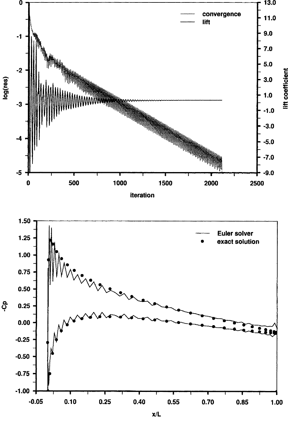
图9.10:绕对称Joukowsky翼型(厚度10%)的二维无黏流动。结构网格,\(M_\infty = 10^{-2}\),\(\alpha = 3^{\circ}\),中心空间离散,显式多级时间推进格式,无预条件。上图为收敛历史,下图为压力系数与精确势流解的比较。图例:上图——convergence(收敛残差,左纵轴为\(\log(\text{res})\))与lift(升力系数,右纵轴),横轴为迭代次数(iteration);下图——Euler solver(欧拉解算器,曲线)与exact solution(精确解,圆点),纵轴为\(-C_p\),横轴为\(x/L\)。
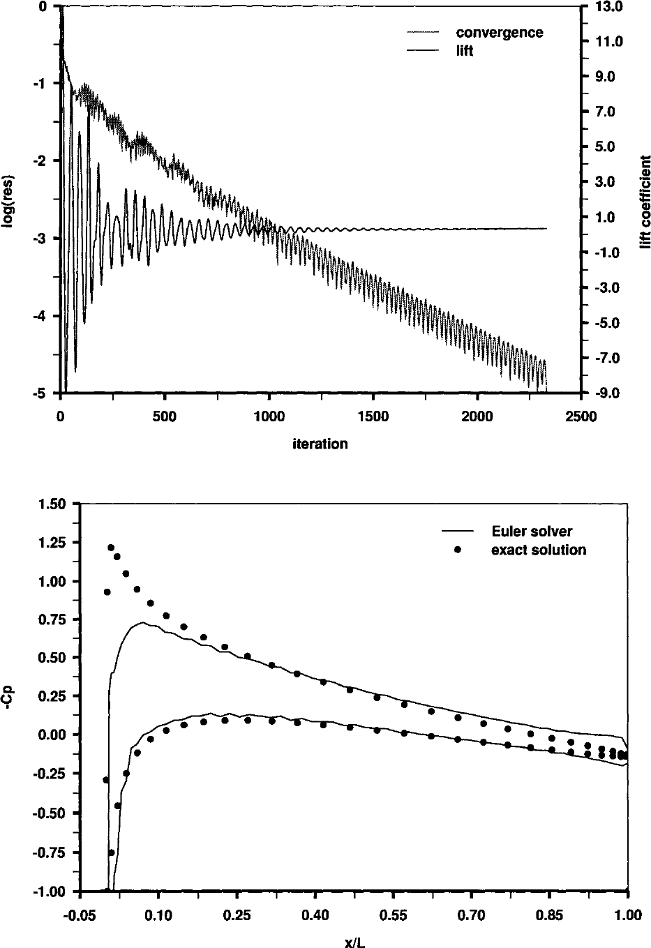
图9.11:绕对称Joukowsky翼型(厚度10%)的二维无黏流动。结构网格,\(M_\infty = 10^{-2}\),\(\alpha = 3^{\circ}\),二阶Roe上风离散,显式多级时间推进格式,无预条件。上图为收敛历史,下图为压力系数与精确势流解的比较。图例:同图9.10。
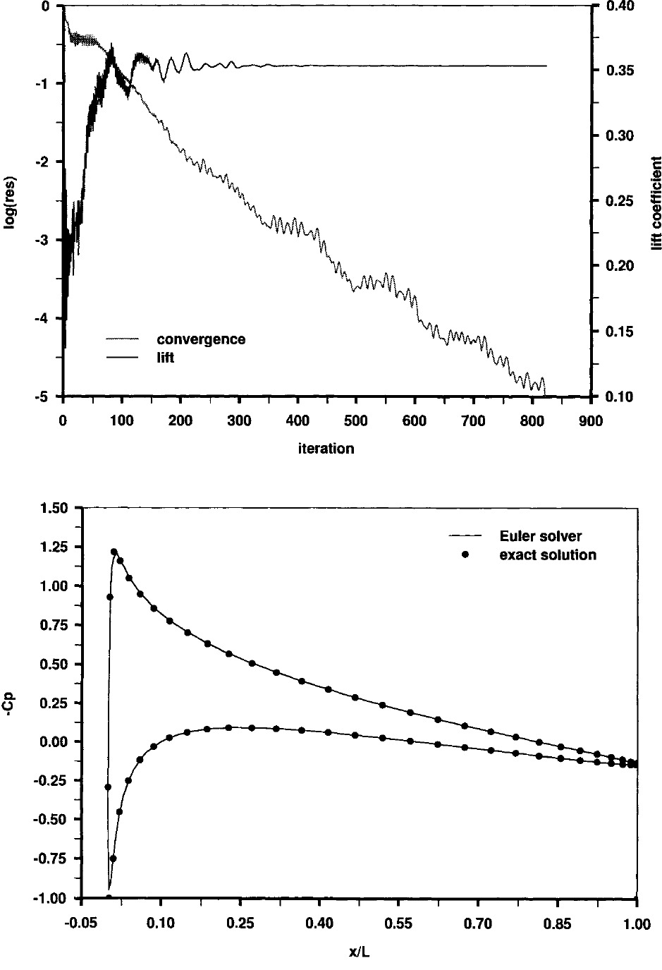
图9.12:绕对称Joukowsky翼型(厚度10%)的二维无黏流动。结构网格,\(M_\infty = 10^{-2}\),\(\alpha = 3^{\circ}\),中心空间离散,显式多级时间推进格式,Weiss-Smith预条件。上图为收敛历史,下图为压力系数与精确势流解的比较。图例:同图9.10。